Main Page/BPHS 4090/In-Vivo Spectrocopy

Required Components

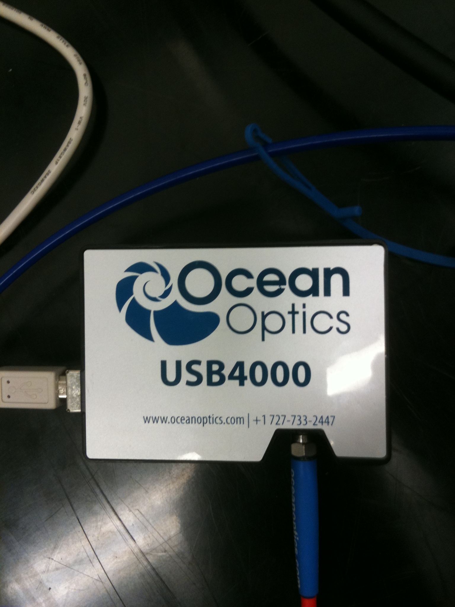
1. USB Ocean Optics spectrometer
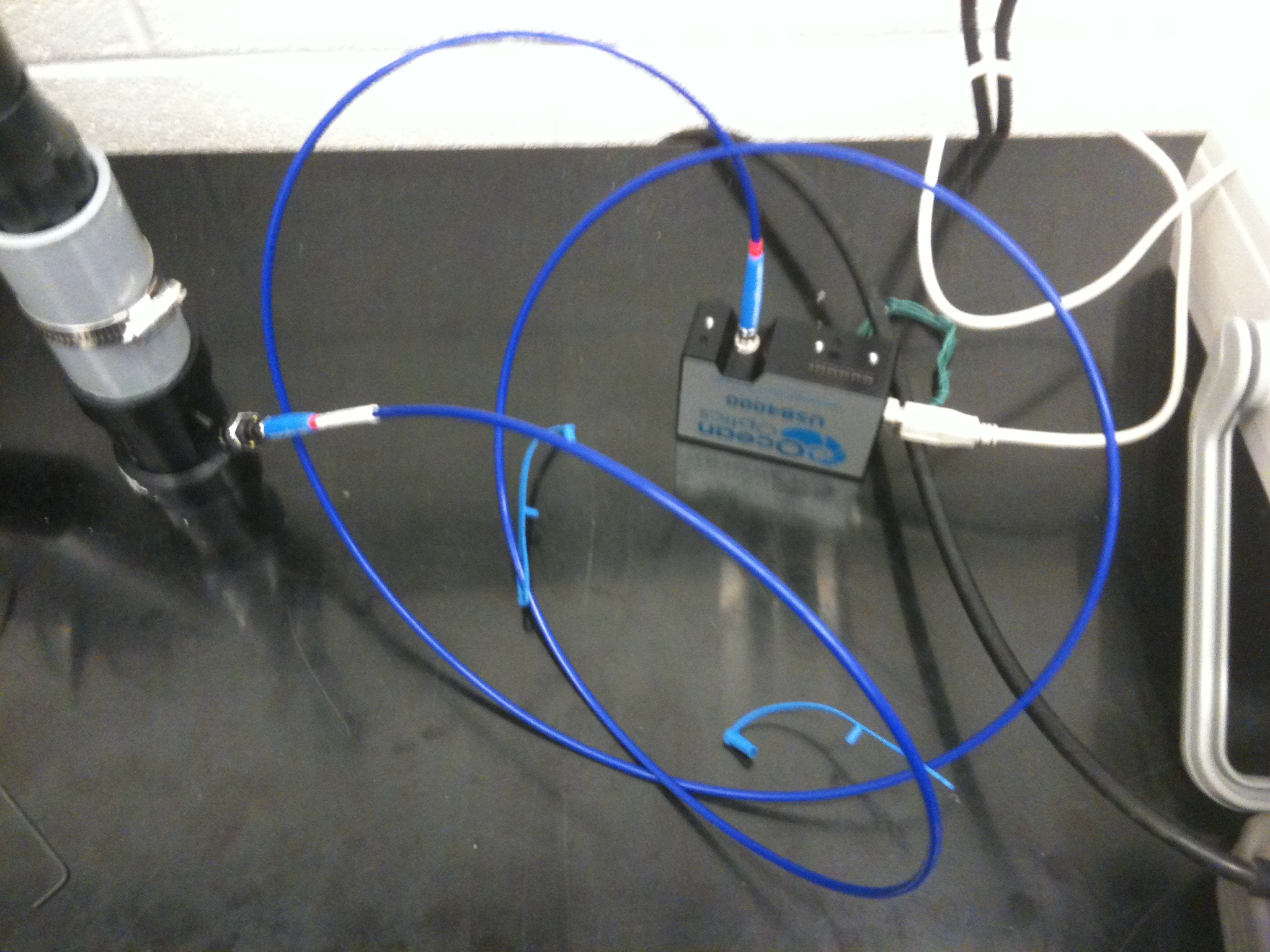
2. Collection fiber for spectrometer
3. PC with spectrometer software and MS Excel (or equivalent spreadsheet) for data processing
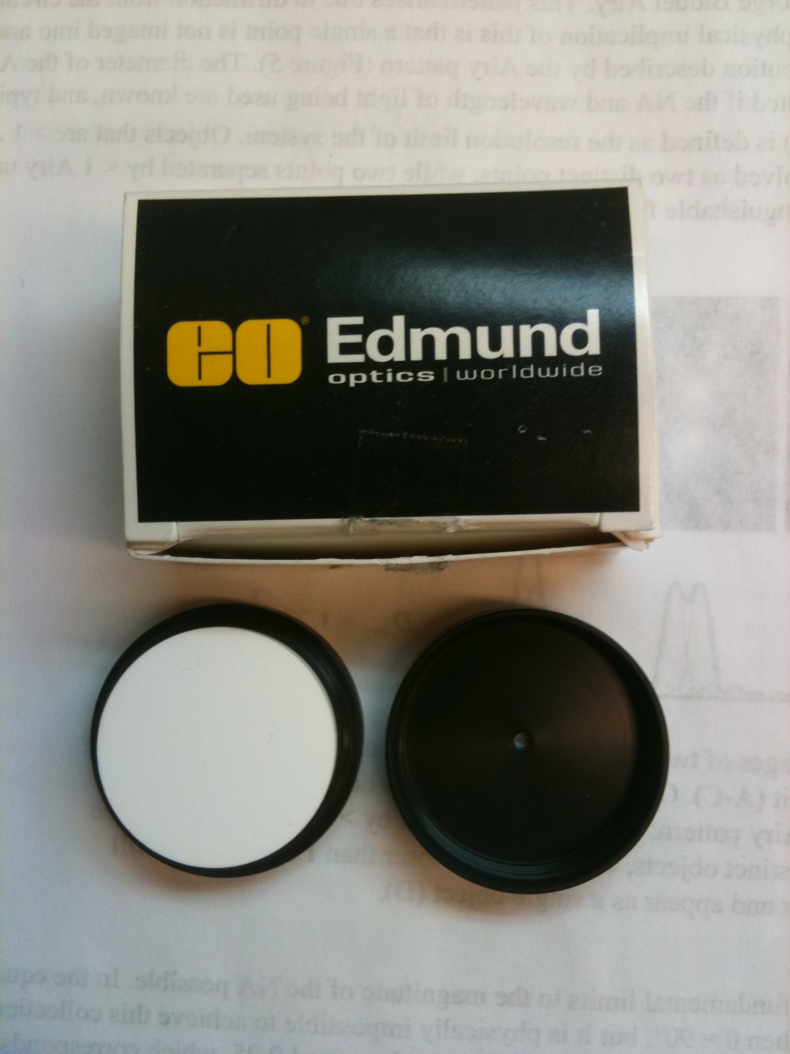
4. White reflectance reference target
5. White LED illumination source
6. Blood pressure compression cuff
7. Excel calculation spreadsheets
8. Stopwatch timer (can use windows clock for this)
9. A usb stick or some way to take your data with you for analysis

Objective

To measure the in-vivo oxygenation state of haemoglobin, and calculate the change in oxygenation before, during, and after reactive hyperaemia by analyzing the colour content of light diffusely reflected off of the skin.

Introduction

Optical methods of skin analysis are ideal because they can be performed non-invasively, and in real-time. It is quite intriguing that so much information can be discovered from something as simple as launching some photons at an object and analyzing what comes back. In this lab, you will be exploring the use of light as a non-invasive measurement tool to determine the in-vivo oxygenation status of haemoglobin in your blood. These measurements will be made in a non-invasive sense, so as much as you may enjoy slicing up your lab partner to get at their blood, it ain’t gonna happen here! You will, on the other hand, have the opportunity to cut off the blood flow to one of your lab partner(s) limbs, though sadly, this will only be temporary. In this lab you will get familiar with the concept of light propagation in turbid (scattering) media, as well as gain experience with optical spectroscopy methods. High resolution spectral information can be analyzed to allow semi-quantitative and fully quantitative analysis of biological materials, and is a very powerful technique, useful for a variety of biophysical applications.

Figure 1 - Absorption spectrum typical for melanin.

Determination of physiologically relevant parameters in a quick, reliable and repeatable fashion is of paramount importance in healthcare and biological research. The optical properties of human skin have been the subject of numerous investigations over the years, and two of the most relevant parameters to measure are the haemoglobin (Hb) oxygenation state and melanin content. Hb and melanin are the two major cutaneous chromophores within human skin, which means that their concentrations are essentially responsible for the colour of your skin. Upon exposure to ultraviolet (UV) light, melatinocytes increase their production of melanin within the skin, we know this process by its more common name, a suntan. The absorption spectrum of melanin is shown in figure 1, and is almost linear over the visible spectrum. It is best measured in the spectral rang above 600 nm, as it is the main source of light absorption in the skin at this wavelength and beyond.

The main target we are after in this lab is the oxygenation state of Hb. Hb is the iron-containing protein attached to red blood cells, and aside from giving blood its red colour, it is responsible for transporting oxygen from the lungs to the rest of the body. The mechanism of oxygen binding in Hb is due to a single iron atom, contained within the protein structure of Hb, and just below a porphyrin ring. A 2D representation of the ring and iron is shown in Figure 2. This structure serves to trap an oxygen molecule and hold it for transport around the body. A typical Hb molecule consists of four of these binding sites surrounded by a protein matrix, and the overall structure of the Hb molecule changes when carrying oxygen. This structural change results in a change in the absorption spectrum of haemoglobin in the 400-600 nm spectral range (Figure 3).

Figure 2 - Schematic representation of the haeme porphyrin ring in Hb.

Figure 3 - Absorption spectra of oxygenated Hb (double peak) and de-oxygenated Hb (single peak).

There is a significant shift of the absorption peak in the 400-450 nm spectral range. However, we will focus on measuring the changes between 500-600 nm since the measurements are easier to perform and more reliable in this range. The absorption spectrum of oxygenated Hb exhibits two peaks in the 500-600 nm spectral range, while the spectrum of de-oxygenated Hb exhibits only a single peak. It is the change between these two states that you will quantify, and to do this we will focus on measuring diffusely reflected light from your palm and the inside of your forearm. These diffuse reflectance measurements will allow us to calculate the absorption spectra of Hb, correct for the effects of melanin from different skin types, and monitor the oxygen saturation state of Hb as we simulate a state of reactive hyperaemia, which is a brief increase in blood flow following a period of ischemia, or arterial occlusion.

Figure 4 - Specular reflection from a surface. Figure 5 - Diffuse reflection from a multi-layer structure.

To understand how we can make measurements of absorption by analysing diffusely reflected light, we should first define what is meant by the term reflection. In general light reflection can be defined in two ways; specular reflection, and diffuse reflection. Specular reflection refers to light that has been directly reflected from an interface, and is directional. A highly polished metal surface, such as a mirror, is an example of a specular reflector. This type of reflector will follow the law of reflection first described by Descartes, namely that the angle of incidence equals the angle of reflection (Figure 4). Another property of a specular reflector is that it will retain image information, which is why you can see your reflection in a mirror.

In diffuse reflection, the light can be thought of as penetrating a small distance into the reflector and scattering multiple times before exiting (Figure 5). This type of reflectance is non-directional, and does not produce any image since all image information in the wavefront is lost due to multiple scatterings. An example of a diffuse reflector would be a piece of white marble. No matter how much you polish the marble, most of the light striking its surface is diffusely reflected, which is why marble makes for a very poor mirror. A perfect diffuse reflector will reflect light uniformly into the 2π steradian space above it, while a perfect specular reflector will reflect light at an angle defined by the angle of incidence. In general most objects will reflect light both specularly and diffusely.

Human skin can also be thought of an object which is diffusely reflective, like the marble, only that it also contains absorbers, namely Hb and melanin. Skin is a heterogeneous, multi-layered structure consisting of three basic layers, each containing numerous sub-layers. The basic layers of skin are the epidermis, which is the outermost layer and provides protection, the dermis, which serves as the location for hair follicles, sweat glands, etc, and the hypodermis, which consists of connective tissue to secure the skin to bones and muscle, as well as blood vessels to deliver oxygen and nutrients to the skin (Figures 6 & 7). Note that it is not important for you to memorize the various layers that make up the skin, but it is important to note where the chromophores we will be measuring reside and originate from.

Figure 6 - Cross section of human skin showing the major layers and components.

Figure 7 - 3D representation of the skins layers and components.

Most of the diffuse reflection you will measure originates from the epidermal layer, which contains no blood vessels or capillaries. The blood diffuses through the dermal layer and into the epidermis, essentially meaning that there is a homogeneous distribution of Hb in the epidermal layer. For the purposes of this lab, you can consider the epidermal layer to be a perfect diffuse reflector, with a uniform distribution of melanin and Hb ‘absorbers’ present in a given volume. Since the diffusely reflected light is interacting with melanin and Hb as it is scattered within the epidermal layer, there is information within this light regarding the absorption properties of Hb and melanin.

Part A: In-Vivo Spectroscopy

Methods

To measure the diffuse reflectance spectra, we will make use of a ‘white’ LED which will be used as an illumination source. The diffuse reflectance will be collected with a fiber optic cable coupled to a computer controlled spectrometer. To simulate reactive hyperaemia, a compression cuff from a blood pressure monitor will be used to temporarily restrict blood flow to the hand. The Hb oxygen concentration will slowly drop following vascular occlusion, and immediately following re-perfusion, you will measure a significant jump in Hb oxygenation, then a steady return to normal physiological levels.

Before getting to the measurements, you should first familiarize yourself with the concept of a spectrometer and how the software interface should be utilized to obtain spectra with a good signal-to-noise ratio. A general schematic for the spectrometer used in this lab is shown in Figure 8.

Figure 8 - Schematic of the light path in the Ocean Optics spectrometer used for this lab.

A spectrometer essentially consists of some light collection optics coupled to an optical fiber (not shown), the light collected by the fiber is passed through a lens and slit assembly mounted inside the spectrometer (2 & 3) before striking a collimating mirror (4). This mirror produces a collimated beam of light, which is then reflected off of a diffraction grating (5) and is focused by a second mirror (6) and onto a linear CCD array (7). A CCD (Charge-Coupled Device) is a light-sensitive detector which produces a voltage proportional to the light striking the active area, or pixels. The diffraction grating will reflect light of different colour at slightly different angles, and thus red light is focused towards the side of the CCD indicated by (8) and blue light is focused towards (9). Reading out the voltage levels on the pixels across the CCD therefore allows us to measure the spectrum of light collected by the fiber. When light is spread across the CCD in this fashion, the wavelength range striking each pixel on the CCD is very small, typically less than 0.25 nm per pixel, which allows for the visualization of very fine spectral features.

Software operation of the spectrometer will be quite basic for our purposes, the software is pre-installed on the PC you will be using for data collection, and can be found under the windows start menu at: Start → Ocean Optics → Spectra Suite. After initialization, the software will be running and ready to collect data. Ensure that you have connected the fiber optic cable between the spectrometer and light delivery/collection housing. The main parameters we will have to change are the exposure, averaging and boxcar settings. Typically it is good to use 4x averaging and 2-4x boxcar averaging. The exposure setting will vary based on the individual, but should be in the range of 200-1000 ms. The ideal gain setting will have the most intense pixel values at ~60,000 levels of grey (see Figure 9).

Figure 9 - Spectra Suite software interface.

Before we are ready to collect data we must first acquire several calibration data sets using the spectrometer to account for the natural spectral shape of the light source and optical system being used (this is the spectrum shown in Figure 10). This will be accomplished by measuring the diffuse reflectance of a ‘white’ reference target, which should have been supplied to you at the start of the lab. This target will allow you to measure the natural spectrum of the LED being used, and this data will later be used to normalize the diffuse reflectance skin spectra and remove any artefacts from the light source and fiber collection system.

Figure 10 - Save Spectrum setup.

collection system. Once you have the proper gain setting for the reference spectrum, open up the save spectrum window (File → Save → Save Spectrum, or hold down “ctrl + alt + s”). The dialogue box shown in Figure *** should appear, and you should fill in the following settings:

1. Under “Save Options” select to “Save every scan”
2. Check the “Stop after this many scans” box, and enter “1” in the box beside it.
3. Under “File Type” select “Tab Delimited”
4. Select your “Save To Directory”
5. Enter “Reference” for the “Base Filename”
6. Ensure “Padding Digits” is set to “5”
7. Hit “Accept”

You should now have a single text file in your save to directory with the reference spectrum data. Now, remove the white reference target and place it back in its container. We are ready to begin spectral measurements. For this you will need the blood pressure compression cuff. Pressure to the cuff is increased by pumping on the bladder, and a silver release valve in front of the bladder allows the pressure to be released. To start the measurements follow the steps below:

1. Open the “Manage Spectrum Exports” dialogue by either going to File → Save → Pause/Resume Export or pressing “ctrl + s”.
2. Highlight any processes and select “Terminate All”
3. Close the “Pause/Resume Export” dialogue
4. Open the “Save Spectrum” window
5. Under “Save Options” set it to save after every 2 scans
6. Check the option to “Pause until started by user”
7. Check the “Stop after this many scans” box, and enter “50” in the box beside it.
8. Under “File Type” select “Tab Delimited”
9. Select your “Save To Directory”
10. Enter “Back of Hand” for the “Base Filename”
11. Ensure “Padding Digits” is set to “5”

The dialogue box should look like this:




Figure 11 - Acquisition parameters for time-series measurements.




12. Hit “Accept”
13. Place the compression cuff just above your elbow, covering you bicep. Ensure that the pressure is fully released by opening the release valve for a few seconds then close it shut.
14. Place the reflectance scan head on the inside of your forearm (you should hold it in place while your lab partner operates the spectrometer software)
15. Optimize the exposure time so that the signal is maximized and no data channels are saturated
16. Ensure that you are using 4x averaging and 4x boxcar
17. Open the spectrum export dialogue by pressing “ctrl + s”

Figure 12 - Manage spectrum exports dialogue.




18. Highlight the process you just set up, which should show its status as “paused”. When you are ready to being, press “Resume All”. Data will now be collecting, and you should begin timing.
19. After 20-30 seconds, begin inflating the pressure cuff to capacity. This will restrict blood flow. The pressure should be maintained to at least 200 mmHg on the pressure dial.
20. After maintaining at least 200 mmHg for 90 seconds of constriction, release the pressure valve to allow blood to re-circulate.
21. Continue monitoring the directory you are writing spectral files into. When you reach file 49 you are done.
22. Press “Terminate All” to remove the completed data capture. If you forget to do this, you will not be able to set up another time series for the next set of measurements. If you find that this occurs, re-open the “Manage Spectrum Exports” dialogue will allow you to terminate the process and use the spectrometer again.

After completing the above steps, repeat them while taking measurements of your lab partner’s inside forearm. After those measurements are completed, record spectra from the inside of your palm, then your partner’s palm. In total, you should have 4 complete data sets, but it may be a good idea to take 2 measurements from each site (8 in total between you and your partner). This way if you find some error during data processing, you have another set to analyze and won’t have to go back to the lab and run the experiment again.

Before leaving the lab please ensure that you have copied all of your data to a usb stick, or emailed it to yourself. You will also need to take with you a copy of the excel macro spreadsheet (.xlm file), which will be used to import all the spectra and calculate everything you need to quantify the change between oxy- and deoxy-haemoglobin. Finally, please ensure that the light source and spectrometer are properly shut down and stored away before you leave the lab.

Using the Excel Analysis Spreadsheet

There is an MS Excel worksheet on the Desktop of the computer called "In-Vivo Spectroscopy Analysis (copy first).xlsm. This was made in Office 2007, but any version of Office should open the file and run the macros. You should set your macro security settings in Excel to run all macros. Copy this file and perform your data analysis using the copy.

1. Copy the Excel Spreadsheet and paste the copy in the directory you created for yourself to save you spectral data collected during the experiment
2. Open this Excel spreadsheet, you will notice there are six sheets of calculations, and 2 charts, but since you haven't imported the data yet, they are blank or show errors.
3. From the "View" tab at the top the window, select the "Macros" icon at the top right.
4. From the list which pops up, select the "ImportSpectralData" macros and click "Edit".
5. You will need to make the following three changes:
   1. Change the entry for Data_Str1 to match the location where you collected your data (ie "Back of Hand000" or "Inside of Forearm000"
   2. Change the entry for Spreadsheet to match the name you gave your copied version.
   3. Change the "DirPath" entry to match the directory where your data is stored.
6. Save the macro by clicking the "Save" icon, and return to Excel sheet by clicking the "Excel" icon
7. While looking at the Main Sheet, select the macro "ImportSpectralData" as before, and click "Run".
8. Data will be imported. It will take a couple of minutes for this process to complete.

Calculation Theory

There are a number of steps that we must perform to normalize the data and convert the reflectance measurements into absorption measurements. These calculations are automatically set up and run in the excel macro for you, but you should understand the steps used and why they are used for answering questions during your experiment write-up. Below we will briefly run through the calculation theory. There are three main calculation steps taken to get the final data once it has been imported into excel.

1. First the recorded spectra are normalized by the reference spectrum from the white reflectance target. This allows us to remove the spectral shape contribution of the light source, which can bias results if not accounted for.
2. Next these spectra must be converted from reflectance spectra into absorption spectra. This is accomplished via the equation shown below, which essentially states that the absorption spectrum of an object is logarithmically related to the inverse of the reflectance spectrum.
3. The absorbance spectra are corrected for the effects of melanin by calculating the slope of the absorption spectrum in the region from 650 – 700 nm. This can be done because the absorption spectrum of melanin is essentially linear across the visible spectrum, and the absorption of haemoglobin is essentially flat in this spectral region, therefore any slope in this region is primarily due melanin concentration within the tissue. For each spectrum is calculated in this region, and the result of the linear fit is subtracted from the spectral data. This step effectively removes the melanin absorption spectrum from the data set.
4. Changes between oxy- and deoxy- states of haemoglobin are related to the single and double-peak spectra of these states. The change between these states can be quantified in a few ways. Here we will employ a very simple method which is based on calculating the slope over two regions in the spectra. This will give us a metric which will be used to quantify the change between oxy- and deoxy- haemoglobin (see figure below).

Figure 13 - Sample spectra of oxygenated and deoxygenated haemoglobin. Dashed lines indicate the slopes being calculated for quantification.

The slope is calculated between 540-565 nm and 565-575 nm, and the difference between these two values gives a measure of the haemoglobin oxygen saturation. As can be seen in the figure above, when the blood is well oxygenated, the slope of the line segments are opposite, and at quite a large angle. In contrast, the slope of the two lines plotted on the de-oxy curve are almost the same value, and of the same sign. Therefore we would expect the value of H(t) to increase as the amount of oxygen is raised in the blood. The actual equation used is shown below, and as you can see it is quite simple mathematically, but it is important that you understand why it is valid to use such a simplified quantification model.

This calculation is performed on each of the spectra you recorded, and the final step now is to generate a normalized haemoglobin oxygen concentration time series from this data. This is done by normalizing the ‘H(t)’ values in the above equation via:

Plotting out H(t)norm as a function of time should then give a plot similar to the one shown below. From this plot you should be able to clearly see the steady decrease in oxygenation as the compression cuff was activated, and a dramatic spike in oxygenation following removal of the pressure and re-perfusion of the tissue with oxygenated blood.

Figure 14 - - Haemoglobin concentration as a function of time during and after a period of vascular occlusion.

Questions/Write up

The following questions should be answered in your notes.

1. What is the main function of haemoglobin in the blood? Briefly describe the physical processes involved in haemoglobin’s biological functioning as well as what happens to the molecule in its various states of oxygenation.
2. How does the presence of melanin affect the data that you have collected and analyzed?
3. Briefly describe the difference between specular and diffuse reflection.
4. Why have we chosen to analyze absorption spectra by reflecting light off of a surface? What are the advantages of performing measurements such as these versus standard transmission spectroscopy?
5. Describe why the oxygen concentration increased so dramatically following the period of vascular occlusion. Is there anything you can say about how blood flows and oxygen is used up in the body on the basis of this data?
6. Was there any difference in your results between the palm of your hand and the inside of your forearm? Please give an explanation for this difference, if you detected any.

The write-up for this lab does not have any specific formatting requirements. In general, you should briefly describe the experiment and the experimental setup to give some background information on what this lab intended to teach you (1-2 pages max). After this, you should describe your data collection procedures as well as discuss your results in the context of the questions asked of you below. The total report should not require more than 4-5 pages. If you wish, you can simply answer the questions in the space provided below. Your write up should answer or address the following questions and comments regarding the work you have done:

1. Include the following plots with your final write up by taking a screenshot in excel and pasting them into your report. All of the values are calculated for you in the spreadsheet, but you must find the areas of max/min haemoglobin using the H(t)norm plot.
   1. H(t)_norm vs time
   2. I(t)_max, I(t)_min, I(t=10s), I(t=_max)
2. Briefly describe how a spectrometer works.
3. Can you suggest any improvements to this experimental setup that would make these measurements easier to perform in a clinical setting? What challenges would a clinical use of this technology face?
4. Why do we have to normalize our collected spectra with the spectrum reflected from the white reference target? What would happen to our measurements if we did not take this step?

Part B: Cytochrome C

Two molecules: hemoglobin, cytochrome c, studied in the lab using the spectrophotometry technique, are shown below. They are members of a large family of metalloporphyrin molecules. The active component of these molecules is the heme group, consisting of the transition metal ion, surrounded by four nitrogen atoms. The heme is part of many proteins, whose functions are diverse and include oxygen transfer and storage (hemoglobin), electron transfer, for example, in cellular respiration (cytochrome) and energy conversion in the photosynthesis process (chlorophyll).

The absorption of ultraviolet and visible light in metalloporphyrins is dominated by electrons located in the conjugated system of carbon bonds in the porphyrin ring and by electrons of the transition metal ion located on the 3d orbitals. The spectrum consists of a very strong transition between the ground electronic singlet (S₀) and the second excited singlet (S₂) at about 400 nm. This is so called the Soret or B band. The weak transition from S₀ to the first excited state S1 is at about 550 nm. This is so called Q band. Due to mixing of states, the probability of transitions from S₀ to S₂ and from S₀ to S₁ is very different. The former is strongly allowed while the latter is only weakly allowed, resulting in dramatically different extinction coefficient for the two wavelengths corresponding to these two transitions. The overlap of the π molecular orbitals of the porphyrin ring with the dπ metal orbitals plays a significant role in determining absorption spectrum of porphyrins. The electric field due to ligands removes the orbital degeneracy of the five 3d orbitals splitting them (typically) into lower lying triplet (hybridized into t_2g orbitals) and higher energy doublet (hybridized into e_g orbitals). Depending on the energy difference between the triplet and the doublet, the ion can be either in high or low spin configuration. When the splitting between the triplet and the doublet 3d orbitals is large (when oxygen is bound to the hemoglobin or when cytochrome c is oxidized) all six electrons of Fe²⁺ occupy the lower triplet with the resultant spin equal to zero. When the splitting between the triplet and the doublet is small, electrons occupy all five 3d orbitals, resulting in high-spin configuration. The overlap between the π molecular orbitals of the porphyrin ring with the dπ metal orbitals is reflected in the slight shift of the Soret band and change of the Q band from a single line (oxyhemoglobin and oxidized cytochrome c) into a closely spaced doublet (deoxyhemoglobin and reduced cytochrome c).

Cytochrome is oxidized by potassium ferricyanide and reduced by sodium hydrosulfite.

We will be using the built-in Absorbance wizard of the SpectralSuite software to analyse the spectrum of cytochrome in the deoxygenated and oxygenated state.

The Absorbance wizard stores in its memory the spectrum of the sample under three different conditions. The first spectrum reading is of the phosphate buffered solution with the addition of either potassium ferricyanide or sodium hydrosulfite. This serves as the control sample. The second spectrum reading is of the sample without the illumination lighting—this therefore measures any ambient lighting that could interfere with the measurements. The final spectrum is of the buffered cytochrome solution with the addition of either potassium ferricyanide or sodium hydrosulfite. The Absorbance wizard stores in its memory the spectrum of the sample under these three different conditions. It then subtracts the first two sample readings from the third sample reading. In this way, the background spectrum is removed from the sample, leaving only the change in intensity of the different reflected wavelengths. A negative change in intensity indicates an absorption.

1. Prepare the control sample, by pipetting 1 mL of phosphate buffered saline into a cuvette. It is important to always hold the cuvette by the top edge so that fingerprints do not distort the spectrometer reading of the sample.
2. Using the scoopula, add about 2 mg of potassium ferricyanide to the buffer within the cuvette. You can use the scale to measure the amount of potassium ferricyanide, however in practice it is only necessary to estimate the amount.
3. Mix the potassium ferricyanide into the buffer by slowly pipetting the solution in and out of the pipette a few times. Be careful to avoid producing air bubbles.
4. Place the cuvette containing the buffer and potassium ferricyanide solution into the cuvette holder of the spectrometer. Turn on the spectrometer illumination source.
5. Next, open the Ocean Optics SpectralSuite software.
6. Under “File” select “New” and then select “Absorbance Measurement”.




7. Select “Next” from the window that appears.
8. Adjust the “Integration Time” so that the entire spectrum appears within the Preview window.
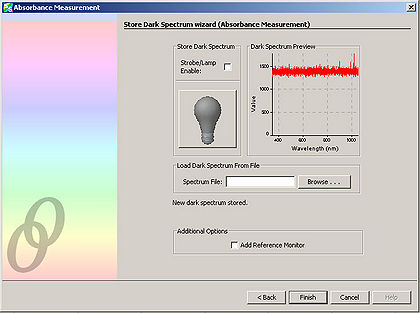
9. Click “Next” and in the resulting window, click the light bulb. This stores the control spectrum in memory.




10. Click “Next”. Block the spectrometer illumination source from reaching the sample. It is important to NOT turn off the spectrometer illumination source, as turning it back on requires additional time to let it warm up. Click the light bulb in the window. This stores the background light in memory.

    
    

    Now prepare the experimental sample. This consists of the cytochrome within buffer with the addition of either potassium ferricyanide or sodium hydrosulfite. This step is performed last because a spectrum measurement of the experimental sample is wanted immediately after mixing the reagents together. (Over time, the effect of the reagents on the cytochrome wears off)

11. To prepare the experimental sample, pipet 1 mL of phosphate buffered saline into a cuvette. Using a new scoopula, add about 1 mg of cytochrome into cuvette. (Typically, this amount is approximated as the smallest reasonable amount of cytochrome that can be transferred using the scoopula). Mix using the same procedure as before (It is crucial to avoid air bubbles!).
12. Next, add about 2 mg of potassium ferricyanide and mix as before.
13. Immediately place the cuvette into the holder of the spectrometer. Select “Finish” on the window. This takes the final spectrum of the experimental sample and automatically subtracts the two background spectrums from before.
14. Repeat this entire procedure but in “Step 12” add 2 mg of sodium hydrosulfite instead of potassium ferricyanide.

A typical absorption spectrum of cytochrome mixed with sodium hydrosulfite.