Main Page/BPHS 4090/microscopy I
Contents
- 1 Required Components
- 2 Objectives
- 3 Introduction
- 4 Methods
- 5 Experiments
- 5.1 Calibration images of micrometer slide & setting CCD exposure
- 5.2 Cheek epithelial cells in brightfield, darkfield and phase contrast
- 5.3 Onion peel slide
- 5.4 (OPTIONAL)Observe brightfield slides using all objectives (10x, 20x, 40x, 100x)
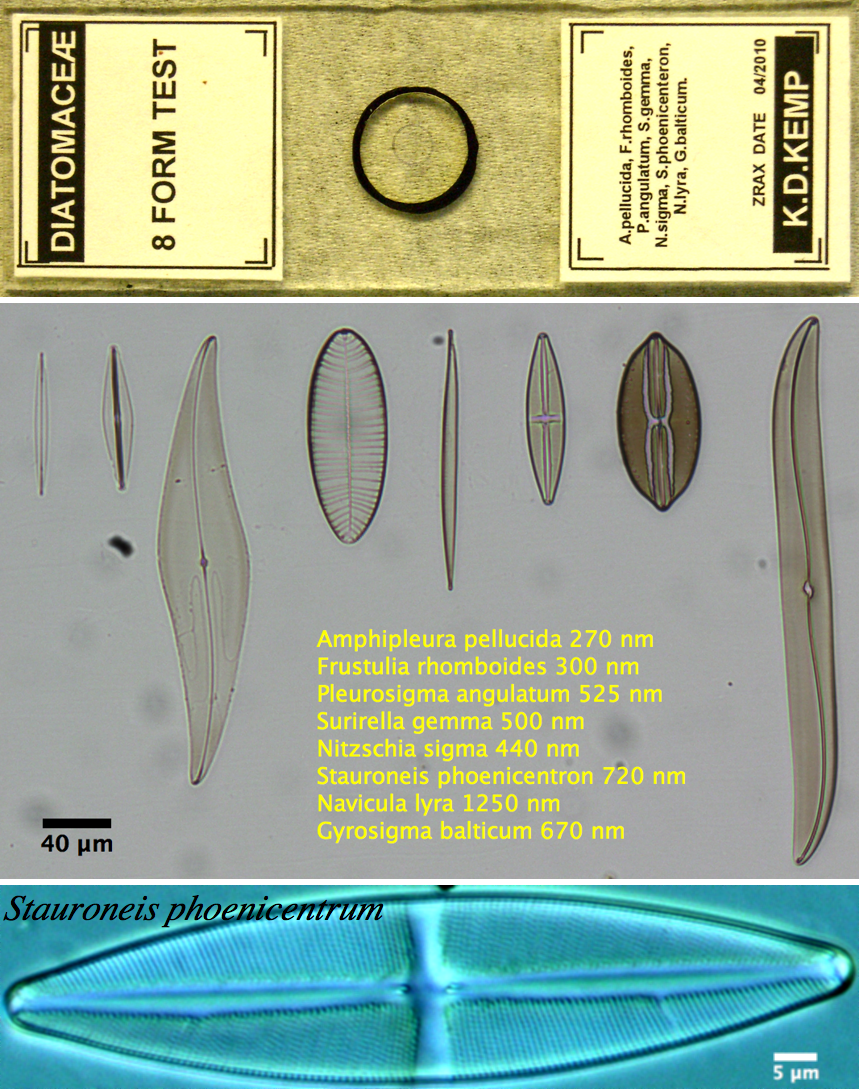
- 5.5 (OPTIONAL) Using the diatom slide as well as the Pap smear slides compare the dry 40x objective with the oil immersion 40x objective
- 6 Questions & Tasks
- 7 Appendix 1 - Background on Microscopy & Optics
- 8 Appendix 2 - Phase Contrast Alignment
- 9 Appendix 3 - Image stack generation and spatial calibration of images
- 10 Appendix 4 - Particle tracking and calculation of particle trajectories
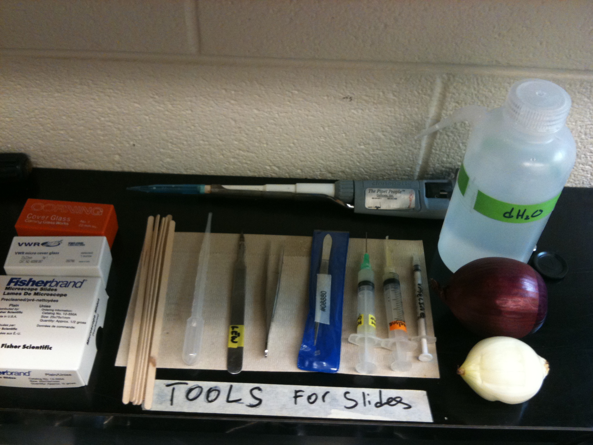
Required Components
- Diatom slide
- Stage micrometer slide
- Stained and unstained baboon eye slides
- Fresh onion
- Knife and tweezers
- Toothpick or popsicle sticks
- Blank slides and coverslips
- Syringe of vaseline with pipet tip end
- Distilled water
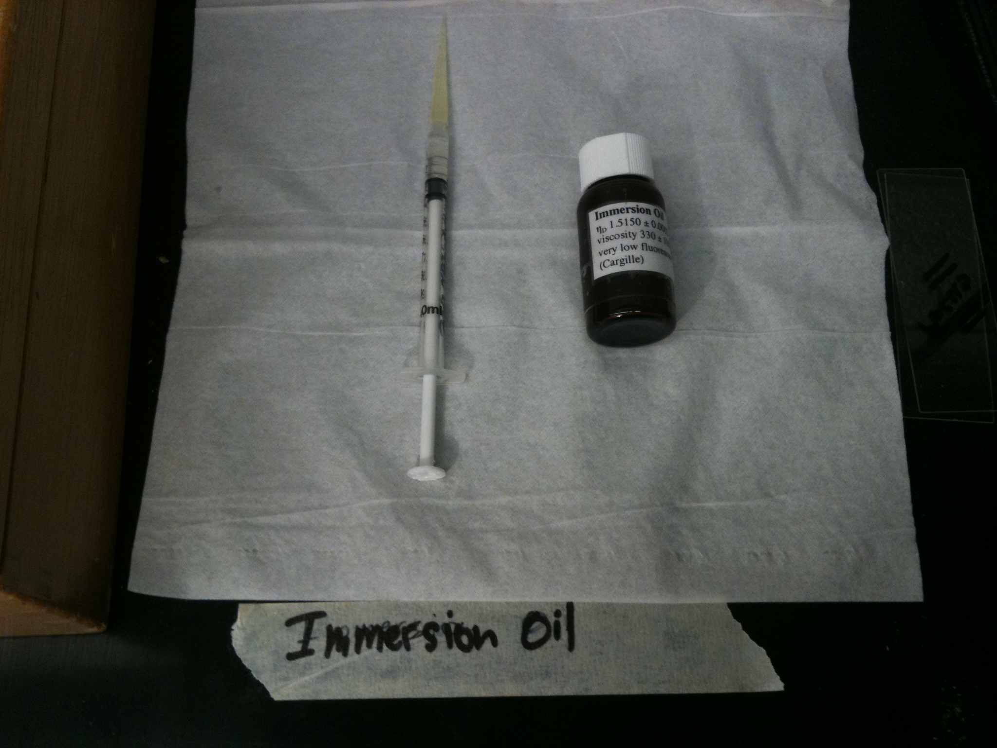
- Immersion oil
- Nikon upright microscope and CCD camera
- USB stick for transferring data and images for processing and report generation
Objectives
Students will get a refresher on the optical light path of microscopes as well as working with digital acquisition software and data processing. Building off of previous knowledge, the students will explore light contrast modes for unstained samples like darkfield imaging and phase contrast imaging. In the first part of this lab these modes will be compared with standard brightfield illumination on stained and unstained specimens. In the second part darkfield imaging will be used to measure the cytoplasmic streaming rate of spherosomes in living onion cells.
Introduction
Imaging has become a vital tool for researchers in virtually all aspects of modern biophysics. Recent advances in microscope technology as well as labelling techniques and gene and protein manipulation methods have led to breakthroughs in our understanding of biological processes. In order to take advantage of these methods you, the biophysicist, need to understand some of the fundamental techniques and concepts in microscopy. You already have experience with microscopes, and this lab will build on that knowledge and get you familiar with more advanced methods as well as working with acquisition software.
The brightfield (transmitted light) imaging mode is something you have already been exposed to. Brightfield imaging mimics the human optical system and is measured in terms of colour and light intensity absorbed by a sample. The contrast method is based off of colour specific absorption of light by the dyes added into the specimen. When working with certain samples, particularly live specimens, the addition of exogenous contrast agents isn’t always feasible as they can potentially interfere with the organism or cells under observation. In this lab we will focus on some specialized microscope techniques to look at unstained samples in a way that lets you observe their morphology without the addition of foreign compounds. The imaging modes you will be using are:
- Brightfield: where samples contain little natural contrast and dyes are added to impart artificial colour
- Darkfield: where photons observed are mostly those that have been scattered by structures within the samples
- Phase Contrast: where optics will be used to visualize changes in the optical path length of samples
A refresher on optical microscopy and imaging theory is included in Appendix 1. Please refer to this section to review some of the fundamental concepts in microscopy. If you feel comfortable with this content you do not have to read through it thoroughly. It has been included as optional background material.
Brightfield Staining
Most biomedical microscopy specimens contain very little intrinsic contrast when viewed directly with transmitted light. For example, to make specimens such as the tissue sections you are using in this lab easier to visualize, stains and dyes are used. These compounds impart additional contrast and enable discrimination of morphological features based on their differential colour absorption across the visible spectrum.
By far, the most common type of stain used in biological microscopy is Haematoxylin & Eosin (H&E). Haematoxylin stains basophilic chemical structures such as DNA in the nucleus dark purple, while Eosin will stain the cytoplasm and extra-cellular regions a shade of pink. When oxidized, haematoxylin forms a structure called haematein. Haematein is a compound that forms strongly coloured complexes with metal ions, most notably Fe(III) and Al(III), and it is these coloured complexes which give the blue/purple colouring seen in the nuclei of H&E sections. H&E staining allows pathologists to observe the density and shape of nuclei in tissue sections, and is the gold standard in the diagnosis of many types of Cancer.
Shown in Figure 1 is a sample of an H&E stained tissue section from a rabbit brain. A low resolution image shows a brain tumour as the dark purple mass, and the zoom view shows the border between tumour and healthy tissue. Note the dark purple staining of the cancerous nuclei, and how densely packed they are.
 Figure 1 - H&E stained section of mouse brain. Shown inset is a zoomed view showing the cluster of nuclei in a
brain tumour (dark purple patch in larger image).
|
Darkfield Microscopy
Dark-field microscopy permits the detection of unstained small biological objects which otherwise provide insufficient contrast under transmitted light observation. In a dark-field microscope a special condenser or aperture stop is used to produce light rays that normally miss being collected by the microscope objective’s collection NA. When this light interacts with a scattering object such as a biological sample, light is scattered into the collection NA of the objective and detected (Figure 2). While it is often the least used of the contrast modes you are exploring, it is relatively simple to adapt a standard microscope for darkfield imaging, and the images produced can be quite striking.
The aperture stop in a darkfield condenser causes light to focus on the specimen in a ‘hollow’ cone. The aperture stop is sized in such a way that this hollow cone is larger than the collection NA of the objective being used, so most of the light put out by the lamp is not detected. Any light that interacts with the sample will be scattered or refracted into the collection NA of the objective being used (light grey region) and detected. Light that does not pass through the sample does not enter the objective’s collection volume, and is thus not detected (gold region).
 Figure 2 - Darkfield illumination path in a typical microscope. An aperture is used to create a ‘hollow’ beam of light
and is focused at the sample. Light that does not interact with the sample (scattering, refraction, reflection, etc) is
outside of the lens NA and is therefore not detected. Light that is scattered or refracted by the sample enters the
collection NA of the objective and is detected.
|
Since there is very little scattering from the glass slides which the samples are mounted on, the image you see appears as a bright image on a dark background, hence the name 'darkfield' microscopy. This microscope method is very useful for viewing small bacteria as well as blood samples. You will also notice that if you are using slides that have not been thoroughly cleaned the dust and dirt on the slide surface will produce a very strong darkfield signal. It is always good practice to clean microscope slides before observation, but this is even more important for darkfield imaging.
An ideal sample to demonstrate darkfield imaging is an onion cell, as it is readily available, cheap, and exhibits quite dynamic activity under darkfield illumination. The endoplasmic reticulum of onion cells forms a network of interconnected tubules within, within which highly refractile objects like mitochondria and sphereosomes are propelled by actin filaments within the cells cytoplasm. An excellent figure depicting the structure and location of this network in an onion cell is found in figure 1 of the paper "Onion Epidermal Cells in Relation to Microtubules, Microfilaments, and Intracellular Particle Movement” by Stromgren-Allen and Brown, which should be provided to you as a separate pdf file (a copy is also stored in the ‘Onion Sample’ folder on the PC desktop). It is recommended that you read this paper as well as “Isolation of Spherosomes (Oleosomes) from Onion, Cabbage,and Cottonseed Tissues” by Yatsu et al, which includes an electron microscope and compositional analysis on the particles streaming around in this tubule network.
Phase Contrast Microscopy
Before getting into details regarding phase contrast imaging we should first review a concept which you should have come across in your studies, the optical path length of an object. It is a relatively simple concept, which essentially states that the optical path length of light traversing an object is equal to the physical length travelled (L) multiplied by the index of refraction (n) of the medium the light is travelling in. Thus, an object can be the same thickness throughout its volume, but changes in the index of refraction make its optical path length vary. Our eyes are sensitive to amplitude (intensity), but not sensitive to changes in light phase induced by optical path length differences. These are the changes we are visualizing in phase contrast imaging.
Optical Path Length = n X L
Phase contrast microscopy produces image intensities that vary as a function of specimen optical path length, with very dense regions (those having large path lengths) appearing darker than the background. Alternatively, specimen features that have relatively low thickness values, or a refractive index less than the surrounding medium, are rendered much lighter when superimposed on the standard (positive) phase contrast (grey) background. Remember; as light travels through a medium other than vacuum, interaction with this medium causes its amplitude and phase to change in a way which depends on properties of the medium (Figure 3). Changes in amplitude give rise to absorption of light, which gives rise to colours. The human eye measures only the energy of light arriving on the retina, so changes in phase are not easily observed, yet often these changes in phase carry a large amount of information.
 Figure 3 - Two parallel light waves beginning perfectly in phase. The top wave travels through a homogenous
optical path while the bottom wave passes through a region where the index of refraction increases (boxed area).
The longer optical path of the bottom wave causes the waves to drift out of phase.
|
In a typical phase contrast microscope the phase variations introduced by the sample are preserved by the instrument, but this information is usually lost in the process which measures the light. In order to make phase variations observable it is necessary to combine the light passing through the sample with a reference wave and take advantage of constructive/destructive interference to highlight changes in phase. The resulting interference between the reference wave and the wave interacting with the sample reveals the optical path structure of the sample as intensity changes in the image observed or captured by a detector. The difference between a phase contrast and brightfield optical path are the addition of two matched phase rings etched accurately onto glass plates within the condenser as well as the objective lens (Figure 4). You can see that the rings are inverse patterns, and they must be aligned co-axially to maximize the phase contrast effect (see Appendix 2 for this procedure).
 Figure 4 - Location of the condenser annulus and phase plate in a PC light path.
|
Methods
A schematic of the microscope you will be using in this lab is shown in Figure 5. You can use this figure as a reference when performing the alignment and configuration of the microscope during the lab. Of particular note is to make sure you have the correct condenser fitted on the scope for this lab, which is the phase contrast condenser (NOT the DIC condenser). For aligning Kohler illumination use the centering screws on the base of the condenser mount (attached to the condenser focus block. For aligning the phase rings use the centering screws attached to the underside of the phase contrast condenser.
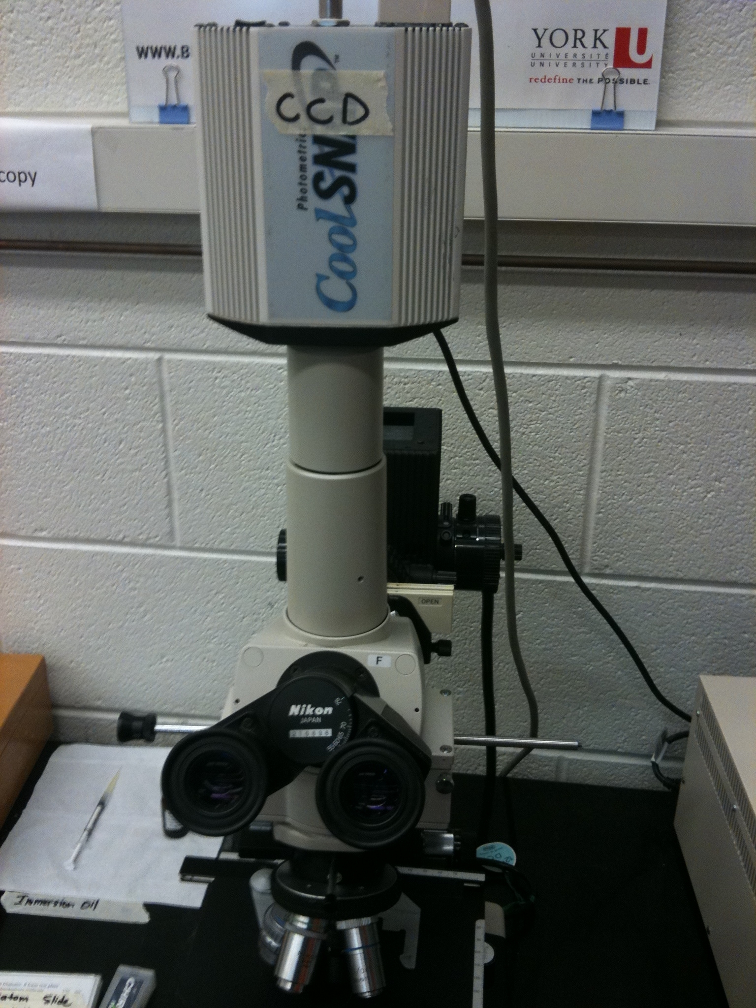
 Figure 5 - Schematic of the Nikon microscope you will be using in this lab. Refer to this figure to familiarize
yourself with the components and their locations.
|
Before performing any measurements or turning anything on, take a moment to study the labelled schematic of the upright microscope you are using. Below are some tips on how to start up the image acquisition software as well as for working with oil immersion objectives.
Initial microscope setup – Kohler illumination
- Familiarize yourself with the microscope and the diagram included in this lab. We will not be using the fluorescence filter cubes or mercury light source for this lab (these will be used in the fluorescence lab).
- Turn on the power to the microscope transmitted light source (power switch is on the base of the microscope).
- Select the 10x objective and select the H&E mouse brain slide and place it on the specimen holder. Focus on the specimen.
- Close the field diaphragm down until you can see its effect in the oculars.
- Focus the condenser until you get a sharp image of the field diaphragm. You may need to gently push the focus block while turning the height adjustment knob as it is a tight at certain points in its travel.
- When the field diaphragm is in focus, you will see a red-blue flare surrounding it and as you open/close the diaphragm you will clearly see a circle getting larger/smaller.
- Now that the condenser height is positioned properly use the adjustment screws on the condenser to center the image of the diaphragm in the field of view.
- Open the field diaphragm so that it is slightly larger than the field of view you are looking at.
- You should now be set up for Kohler illumination which illuminates the sample with a
uniform field of light. An example showing poor contrast and colour reproduction
caused by non Kohler illumination is shown below for reference:
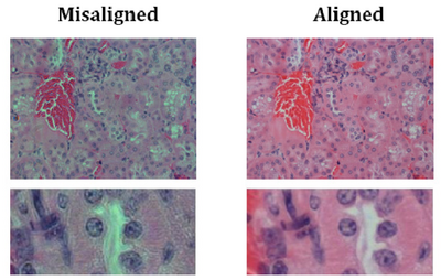
- If you change to a different objective you may need to re-adjust the diaphragm size or condenser height for optimal performance, but in general you should be ok for the rest of the lab.
- When aligning the phase contrast mode the Kohler illumination could shift slightly along X & Y, which should not matter much as long as the condenser height is ok and the aperture is opened slightly larger than the field of view.
Working with immersion objectives
- When working with immersion objectives be very careful with how much oil you use and clean the objective thoroughly when finished.
- Also be careful not to get any oil on the non-immersion objectives. If this does happen, remove the objective from the microscope and clean it with the lens cleaning solution. Remove one of the microscope's eyepieces and use it to examine the lens and ensure it is clean. Use the lens to look at a specimen to confirm it is clean. If it is still dirty, repeat the cleaning procedure.
- Move the stage down and use the light from the condenser as a reference for where to place the drop on the specimen. You don’t need much immersion oil here, if you use too much it will be a waste and make it more difficult to clean the slide when you are finished.
- Carefully finish rotating the 100x or 40x objective in place and re-focus on the sample. At this point you can freely move around the slide, just try and keep the X-Y motion of the sample to a slow and steady pace or else you will lose oil quickly and have to add more. If you make slow, controlled motions the oil will not spread out as much.
- After acquiring your images, lower the stage and remove the slide. Carefully clean the slide and lens using a kimwipe and the supplied cleaning fluid.
- When you are finished with the lab thoroughly clean any immersion objectives used as well as slides that are part of the permanent lab (ie, micrometer, diatom slide, stained slides). This is a critical step, as over time oil that is not cleaned can degrade image quality and even render the very expensive objectives on the microscope useless. The objectives will unscrew from the turret, and using one of the eyepieces you can examine the lens after cleaning it to ensure there is no residual oil (ask your lab instructor to show you how to do this if you are unsure).
Getting ready for acquisition and digital image capture.
- Turn the CCD on by pressing the power switch located on the top of the camera.
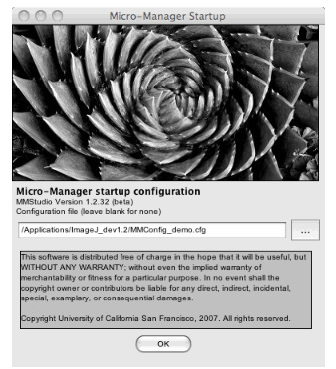
- Launch the μManager software which will allow you to record data and adjust the
camera gain. Upon startup select the default configuration file in the splash screen that
starts up.
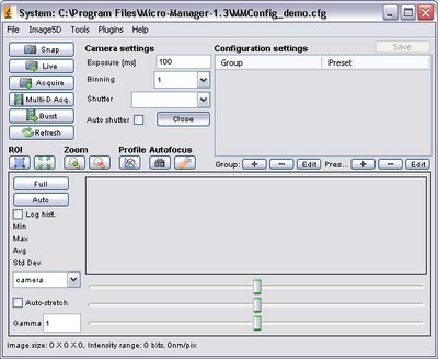
- After startup, the main control screen for μManager should appear. From here you can
change the exposure settings on the CCD camera to optimize the signal by typing in an
exposure time (the units are milliseconds).
- Rotate the eyepiece mounting block to the left to allow light to pass through to the CCD camera.
- Pressing the ‘live’ button in μManager should open a new window that shows a live image of the light striking the CCD camera.
- Pressing the ‘snap’ button will take a single snapshot which you can then save for later processing.
- Pressing the ‘Multi-D Acq’ button opens the multi dimensional acquisition dialogue from which you can configure a time lapse acquisition (see below).
Setting up a timed acquisition in μManager
- For some experiments you will want to set up a timed acquisition so that you can make
a movie and dynamic measurements of samples. To do this open the multi-dimensional
acquisition dialogue and refer to the figure below to set relevant acquisition
parameters.
- Number = number of frames you want to acquire
- Interval = time between frames (for setting up time-lapse)
- Save Images = directory to save your images to (files will be automatically
numbered and timestamped)
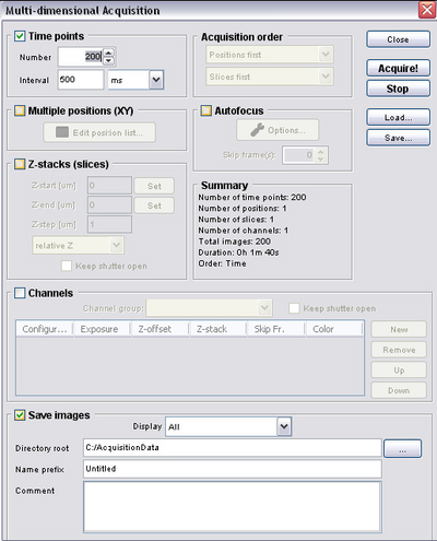
- It is a good idea to include parameters such as the CCD exposure time, microscope objective, time delay and CCD bin settings in the file name or folder.
- Be sure to change directories and file names between movies to keep the organization of the files neat.
- Pressing the ‘Acquire’ button will initiate the acquisition protocol using the parameters you specified and the CCD gain currently being used.
- Double check the folder after acquisition is complete to ensure all the files were properly saved.
- For some experiments you will want to set up a timed acquisition so that you can make
a movie and dynamic measurements of samples. To do this open the multi-dimensional
acquisition dialogue and refer to the figure below to set relevant acquisition
parameters.


Experiments
There are a number of small exercises to be performed in this lab. The first few are relatively straightforward, and shouldn’t take a significant amount of time to finish. Getting the onion peel sample prepared correctly may take a few tries, and finding the most active cells and recording the image sequences will also eat up a fair bit of time. If you do complete everything early, there are a number of additional slides which you can look at in the slide cases.
First, set the microscope up for Kohler illumination, and follow the directions in Appendix 2 for setting up the phase contrast alignment. Once you are finished with that, start by taking some images of the stage micrometer so you can spatially calibrate the images. This will later allow you to make measurements of object sizes and calculate cytoplasmic streaming speeds in the onion cells. Follow through the steps and tips below.
Calibration images of micrometer slide & setting CCD exposure
- Acquire and save images of the metric scale using the 10x, 20x, 40x (air and oil), 100x oil objectives.
- Acquire the oil immersion images last, and ensure there is no oil on the slide when using the dry objectives.
- Please ensure the slide is cleaned thoroughly and placed back in its case after you are finished with it.
- Place the micrometer slide on the microscope and rotate the eyepiece turret counter clockwise (to the left if facing the microscope) to allow the light to pass through to the CCD camera.
- Note the CCD camera has an additional 2.5x doubling lens in front of it. Thus a 10x image to your eye is magnified up to 25x on the CCD. In other words; the field of view you see with your eyes when using a 100x objective is what the camera sees when using the 40x objective.
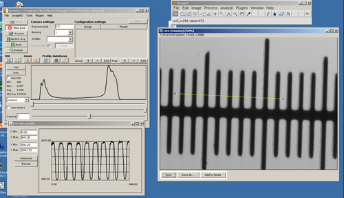
- Press the ‘Live’ button and prepare to adjust the CCD exposure setting.
- Adjust the CCD exposure setting so that you get as bright an image as possible without saturating the CCD pixels. You can tell when you have a good exposure setting by observing the histogram in the lower portion of the μManager window.
- Click on ‘Full’ and you will remove any digital contrast adjustment from the live display. Set the exposure time so that the histogram in the graph window is properly exposed like the example below (depending on your sample you may not see two separate peaks as shown).
- You can use the slider bars to set the black and white levels of the image (applying contrast), but it is always best to start by displaying the full data range.
- When you are happy with the exposure setting you can press the ‘Snap’ button to take a single image which will open in a separate window. You can then save this image for later processing in ImageJ.
- Use the objective magnification in the file name to make it easier for you to correlate the proper calibration images with the data you will need to calibrate. You will calibrate the images after completing the experiments. Importing images sequences and applying spatial calibrations in ImageJ is covered in Appendix 3.
Cheek epithelial cells in brightfield, darkfield and phase contrast
- By gently scraping a toothpick on the inside of your mouth you will remove a large number of epithelial cells, which are ideal to demonstrate the difference between the imaging modes being explored in this lab.
- Transfer the material you scraped off to a glass slide.
- Apply a thin bead of vaseline to the surface of a microscope slide, forming a square approximately 1 cm2 in area around the cells.
- Place a small drop of distilled water in the centre of the vaseline square.
- Place a coverslip on top of it all and gently press down on it to seal the specimen. This should prevent drying out of the cells during the experiment.
- Observe the cells in darkfield, brightfield and phase contrast (Note; only the 10x objective is equipped for phase contrast imaging).
- Acquire images in each of these modes and compare them on the computer monitor to see how the same structures appear visibly different depending on the technique used.
- Try to go for cells that are not folded and avoid cells that are clumped together. If the cells are too tightly packed it is easy to prepare another one.
- Most of the cells you will observe are dead or dying, which is why they come off so easily. This makes them somewhat un-interesting for time-lapse imaging, but the onion cells show significantly more activity.
Onion peel slide
- By cutting into an onion and carefully removing a thin transparent sheet of cells from the interior layers we can catch some dynamic events.
- After removing the onion peel, lay it flat on a microscope slide using tweezers and toothpicks to gently pull it flat. It may help to put a small drop of water on the slide first if you find that the peel is tearing easily because it sticks to the slide surface.
- Cut the peel to approximately 1 cm2 and apply vaseline around its border.
- Place a drop of distilled water on the sample.
- Seal with coverslip.
- Observe in darkfield first using the 10x objective.
- Fresh and healthy cells will have an intact cell wall, and clearly defined nucleus with quite fast and dramatic streaming. Move around the sample looking for cells exhibiting cytoplasmic streaming. You may need to switch to the 20x or 40x objective to see the streaming better with your eyes.
- If you don’t see any activity in this slide, make up another one from a different layer in the onion. It may take several tries to get a fresh one. There is a sample movie in the ‘Onion Sample’ folder on located on the computer desktop to demonstrate the type of activity you are looking for. The movie was captured at 1 frame per second and accurately shows the streaming speeds you should see when using the 10x and 20x objectives and the CCD camera. The 10x movie is what you would see using 25x when looking with your eyes, and the 20x movie is equivalent to 50x when looking with your eyes.
- Try and find a cell away from any air bubbles or very bright objects.
- Record movies of the cytoplasmic streaming using the 10x/Ph2 in transmitted light, phase contrast and darkfield, as well as the 20x objectives which has no phase plate and thus cannot image in phase contrast mode.
- Open the ‘multi-dimensional acquisition’ window and select a folder to save your data to. Be sure to indicate which objective you used in either the folder or file name.
- Acquiring 100 frames with a delay of 500 ms between frames should be more than sufficient.
(OPTIONAL)Observe brightfield slides using all objectives (10x, 20x, 40x, 100x)
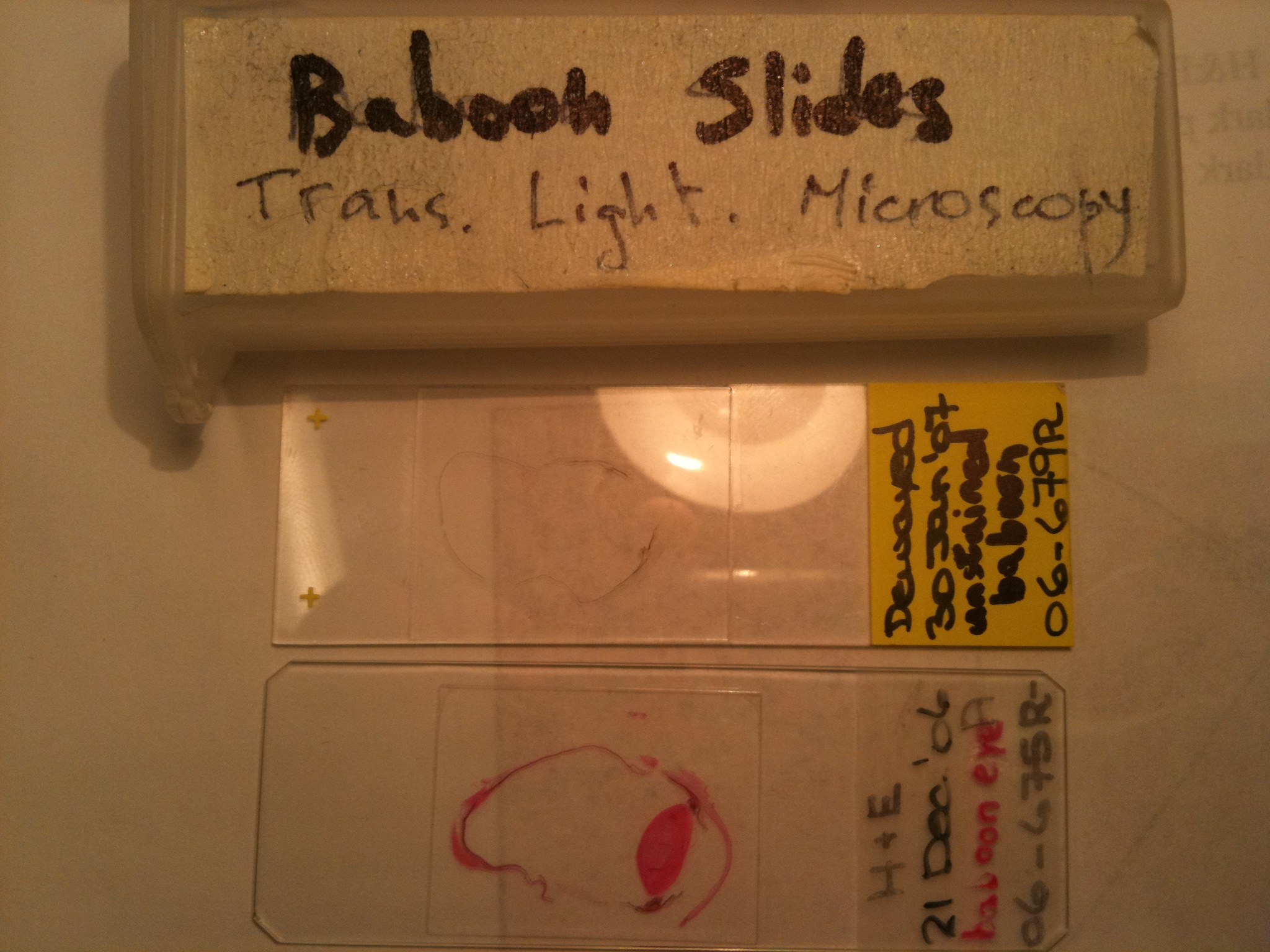
- Stained and unstained sections of a baboon eye should be provided to you by your instructor.
- You can clearly make out cellular structures, including the retinal layers opposite the lens in the stained section. In the unstained section you will not see much other than some natural pigments in the retinal layers.
- You will also be provided two Pap smear test slides as an example of healthy and diseased samples. Note the change in nuclear morphology between the samples. Which sample looks ‘healthier’ to you?
- A number of other slides are in the containers for you to explore and image if you have time to come back to them. A list of what the specimens are and what stain was used to prepare them is included in an Appendix 5.
(OPTIONAL) Using the diatom slide as well as the Pap smear slides compare the dry 40x objective with the oil immersion 40x objective
- Focus on the sample using the 40x dry objective.
- Switch to the ‘Live’ view on the CCD and adjust the exposure setting for the 40x dry objective.
- Rotate the dry objective out of the way and place a drop of oil on the slide and rotate the 40x oil objective into place. Re-focus and observe the sample through the eyepieces.
- Do you see more detail with the one of the lenses? Explain why this is so.
- Switch back to the ‘Live’ view on the CCD. What is the effect of NA on the CCD exposure as well as image contrast?

Questions & Tasks
- Why do we use Kohler illumation? What is the major advantage of this illumination setup?
- Briefly describe the difference between darkfield and brightfield and phase contrast imaging.
- How does the NA affect lateral (X-Y) resolution on images? Is there any effect along the Z (focusing) axis?
- Describe why oil immersion lenses produce sharper images as well as some of the things to be cautious about when using immersion optics.
- Calibrate the images you acquired and generate image stacks using the method described in Appendix 3.
- Calculate the cytoplasmic streaming rate in the onion cell using the method described in Appendix 4 and compare with the value reported in the Stromgren-Allen & Brown paper.
- You can create a movie of your cytoplasmic streaming data sets by saving your stack as an AVI file within ImageJ (select ‘File’ -> ‘Save As’ -> ‘AVI’). Using a framerate of ~ 2 will show the particles moving in real time. Also create movies running at 8 fps (4x real time) to see a much more dynamic version of the streaming.
Appendix 1 - Background on Microscopy & Optics
The most basic function of any microscope is to magnify an image and enhance the resolution visible with the naked eye. In general, increasing magnification also increases the resolution when the optical system being used has been designed and aligned properly. Before getting into specifics, let’s review some fundamentals of how lenses and light form images.
 Figure 1 - Imaging properties of a single thin lens. The location and size of the image produced can be calculated
via the lens maker’s formula and the magnification ratio.
|
The simplest way to produce a magnified image of an object is with a single lens, such as a magnifying lens. Figure 1 shows a diagram that most of you should have seen at least once in your university career, it is of a single ‘ideal’ thin lens and shows how light from the top of an object is translated to an image plane by a lens with focal length ‘f’. Using the lens maker’s and magnification formulas in the figure, the location and size of an object can be calculated if the focal length and object size/position are known. When an object lies at a distance of 2f from the lens, the image is formed at -2f and the magnification factor is -1 (ie, the image is inverted). As the lens is moved closer to the object (decreasing dobj), the image distance and magnification increase.
It is this image forming principle that is the basis for optical microscopes. The most basic form of microscope, the compound microscope shown in Figure 2, contains two lenses. The objective lens which collects light from the sample and the eyepiece lens, which further magnifies the image generated by the objective and translates it to the back of the eye, or a detector such as a CCD camera.
 Figure 2 - A simple compound microscope that can be used to produce a magnified image of a specimen. The
dotted line represents the apparent image size as seen by the observer or detector.
|
In reality, each of these ‘lenses’ shown in Figures 1 & 2 are made up of a number of optical components with differing shapes and glass compositions. A single lens is typically shown in the figures to represent a multi-element lens, as diagrams can get very complex if this is not done. The use of multiple lenses in a compound microscope allows a larger magnification factor to be achieved, and also allows for corrections of image distortions (aberrations) which degrade image quality when not properly corrected. A discussion of aberration correction and optical design is beyond the scope of this lab and most undergraduate coursework, thus we will not go into this in depth.
 Figure 3 - Numerical Aperture (NA) is a measurement of the collection volume of a lens. In the figure, D represents
the lens diameter, f the focal length of the lens, n the index of refraction of the surrounding medium, and θ is the
maximum collection angle of the lens.
|
Along with its magnification factor, the Numerical Aperture (NA) of an objective lens is very important in reproducing sharp features in a specimen. The NA is a measure of the cone of light collected from an objective lens; a higher NA indicates a lens that is more efficient at light collection and produces a smaller focused spot size, which translates into better image contrast and resolution. A diagram of the NA measure is shown in Figure 3. Light is focused to a point which is one focal length from the lens centre. If the lens diameter is defined as D, then the maximum collection angle of the lens for an on-axis point is then θ = tan-1(2f/D). The NA of a lens is defined as NA = n x sin(θ), where n is the index of refraction of the medium between the lens and the sample.
 Figure 4 - Focused spot size dependence on NA. As the NA is increased the collection volume increases and the
focused spot size gets smaller. This allows higher NA objectives to see finer details with better resolution and
sensitivity.
|
As the NA is increased, the size of the focused spot decreases and the optical resolution increases (Figure 4). Strictly speaking however, the distribution of the focused spot is not actually a ‘spot’ but an Airy pattern, named after George Biddel Airy. This pattern arises due to diffraction from the circular aperture of the lens, and the physical implication of this is that a single point is not imaged into another single point, but into a distribution described by the Airy pattern (Figure 5). The diameter of the Airy pattern (DAiry) can be calculated if the NA and wavelength of light being used are known, and typically ½ of this value (Airy Radius) is defined as the resolution limit of the system. Objects that are > 1 Airy unit apart will be clearly resolved as two distinct points, while two points separated by < 1 Airy unit will blend together and be indistinguishable from one another in the final image.
 Figure 5 - Images of two closely spaced objects as they approach the Airy resolution limit (A-C). Optical resolution
can be defined in terms of the width of the Airy pattern; two points separated by > 1 Airy radius will be resolved as
distinct objects, while objects closer than 1 Airy radius will blend together and appear as a single object (D).
|
In practice, there are some fundamental limits to the magnitude of the NA possible. In the equation for NA, sin(θ) is maximized when θ = 90°, but it is physically impossible to achieve this collection angle in the real world. The largest NA possible for ‘dry’ objectives is around 0.95, which corresponds to a collection angle of θ ≈ 72°. To further increase the NA beyond 0.95 a ‘wet’ or immersion objective is used. Increasing the index of refraction (n) of the region between the lens and the sample also increases the NA, and typical immersion fluids are water (n ≈ 1.33) and oil (n ≈ 1.55). While increasing the NA reduces the spot size, allowing smaller features to be resolved, it also increases the light collection efficiency, thus improving the signalto- noise ratio in images. Immersion optics are more difficult to work with, but they offer unmatched resolution and image quality, as we will see during this lab.
Appendix 2 - Phase Contrast Alignment
This section gives an overview of the steps required to properly alight the phase plates in the condenser and objective.
- Place a brightly stained specimen on the stage and rotate the 10x/Ph2 objective into the optical pathway with the condenser on the BF setting. Follow the Kohler alignment procedure from the main part of the lab.
- Remove the sample and place a blank microscope slide on the stage.
- Rotate the condenser turret into the Ph2 position.
- Remove one of the microscope eyepieces and replace it with the phase telescope (if it is not with the microscope, it will be in the wooden box that holds the DIC condenser).
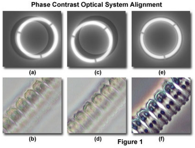
- While looking through the phase telescope, adjust its focus (slide it in and out of the tube) until the phase plate in the objective is in sharp focus (it will look something like Figure 1a & 1c).
- Locate the condenser annulus centering knobs and adjust the position of the annulus until it is overlapped with the objective phase plate (Figure 1e). Note: do not attempt to adjust the position of the condenser annulus with the main condenser centering knobs (the ones you used for Kohler illumination). This effort will probably not achieve the intended condenser annulus alignment and may compromise Kohler illumination.
- The microscope should now be properly configured for phase contrast.
- Take your prepared cheek cell sample and place it on the microscope.

Appendix 3 - Image stack generation and spatial calibration of images
- Using images acquired as well as the stage micrometer images we will now generate an image stack, which will allow you to quickly or slowly go through the data set frame by frame. Also, the micrometer images will be used to spatially calibrate the data set.
- Open the folder containing your data set and highlight all of the files you wish to open.
- Drag all of the files onto the ImageJ program box (Important: to make sure the files import in the correct numerical order make sure your mouse is on the first file when initiating the drag and drop to ImageJ).
- To turn the images into a stack click the ‘Image’ menu in ImageJ and select ‘Stacks’ then ‘Images to Stack’. This should combine all the separate image windows into a single window. Moving the slider at the bottom left or right will play the sequence as a movie, or you can go frame by frame.
- Open the micrometer calibration image corresponding to the objective used to acquire the stack that was just created.
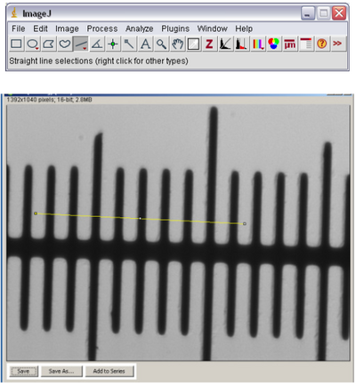
- Using the line tool in ImageJ (see below) draw a line across the marks on the slide. The lines
on the slide are separated by 10 microns, so measure from the leading edge of one black bar
to the leading edge of another bar across the field of view.
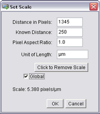
- Open the ‘Analyze’ ImageJ menu and select ‘Set Scale’. The following window should pop
up, and already have the length of the bar you just drew (in pixels) filled in as the first entry.
Input the known calibration distance based on the number of dashes traversed by the line
and select the units to be microns. Also, check ‘Global’ to apply this calibration to all
opened images, including your stack.
- Save and close your stack, then repeat with the rest of your images. Record the numbers for each objective as you only have to measure the calibration once, and then can fill in the numbers manually in the ‘Set Scale’ dialogue.
- If you want to create a movie of your data stack select ‘File’ -> ‘Save As’ -> ‘AVI’. Selecting a framerate of ~ 10 frames per second will be roughly 5x real time. These files can be played in any computer media player.


Appendix 4 - Particle tracking and calculation of particle trajectories
- Open an image stack from your onion cell data set taken in darkfield and ensure it is calibrated properly.
- Scan through the movie and try and identify a particle that stays in focus for at least 10 consecutive frames and can be clearly identified in each of them.
- You can zoom in and out using the ‘+’ and ‘-‘ keys on the keyboard. You will find it easier to track the particles if you zoom in a bit.
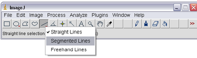
- Select the ‘Segmented Lines’ tool from ImageJ by right clicking on the line tool icon as shown
below. This will allow you to left click on the particle in each frame and ‘draw’ its trajectory
on the stack. Double clicking will end drawing of the line.
- Using the segmented line tool click on the centre of the particle you want to track. Using
the ‘<’ and ‘>’ keys on the keyboard you can scroll through the image stack frames. Track
your particle into the next frame and mark it again with a single left click, it should have
moved 10-12 microns. Repeat until the particle drifts out of view or becomes lost, ending
with a double click to finish the line draw procedure.
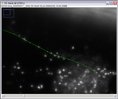
- The number of boxes in the line segment indicates how many frames you tracked the particle for. Count the number of frames you went through and call this number Δf.
- Now select ‘Analyze’ and then ‘Measure’ and a text box should pop up. The last entry in this box should tell you the length of the line you just drew in microns. Call this Δd.
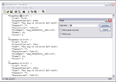
- To get the time taken, we need to confirm the time between frames from the metadata
which μManager exported while acquiring data. In the folder containing your data set there
should be a file called metadata.txt. Open this in wordpad and do a find for the highest
frame number acquired. Ie, if you set up the multi dimensional acquisition to take 100
frames, search for ‘100’. It should look like this.
- Now, take the elapsed time (in ms) and divide it by the number of frames acquired to get the time scale of your data set calibrated, call this value Δt.
- The average speed your particle is moving at is therefore:
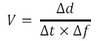
- Repeat this calculation on multiple particles (~10) to get an average value from your data set.


