Main Page/BPHS 4090/microscopy II
Contents
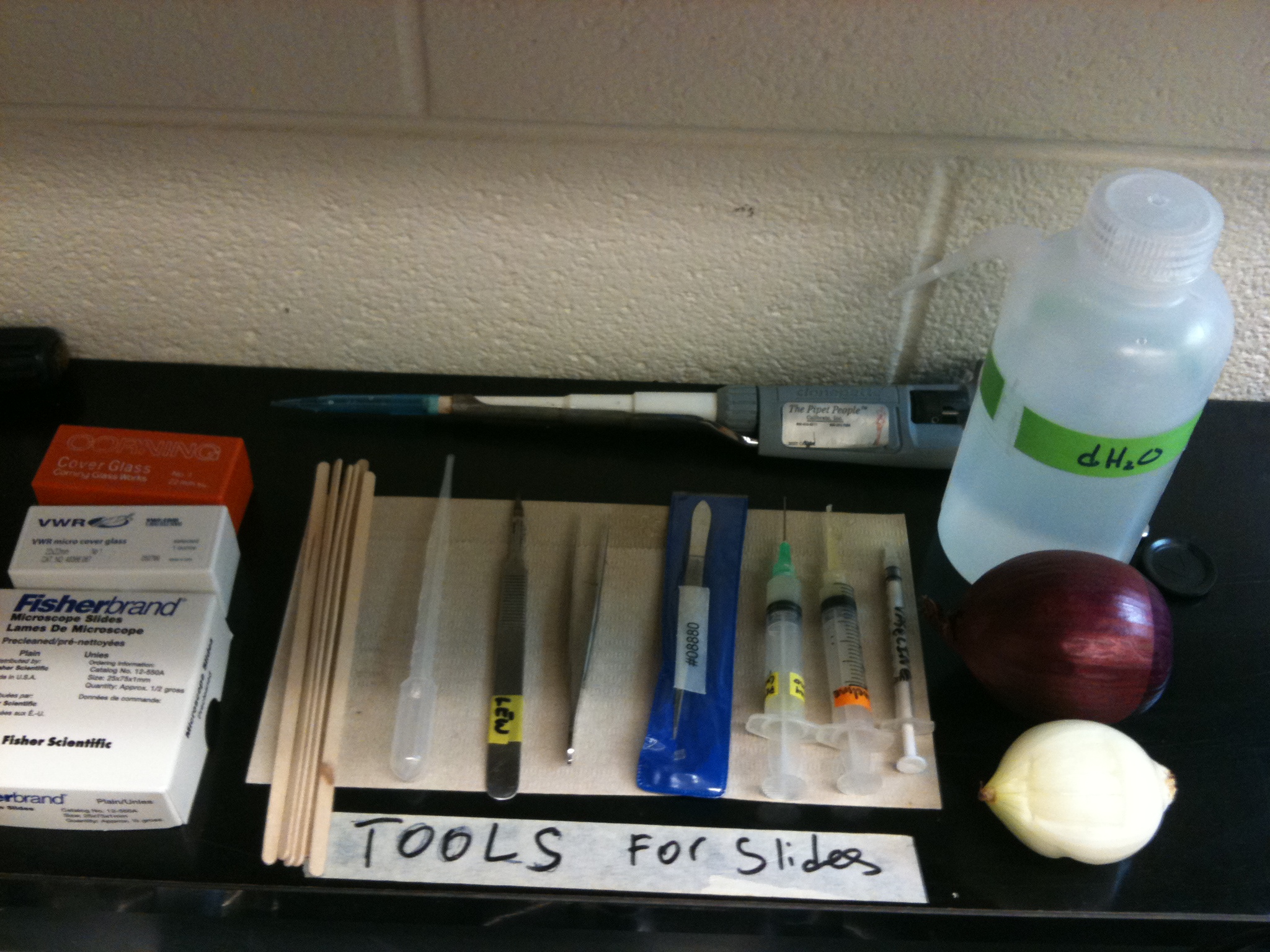
Required Components
- Stage micrometer slide
- Chroma fluorescent slide kit
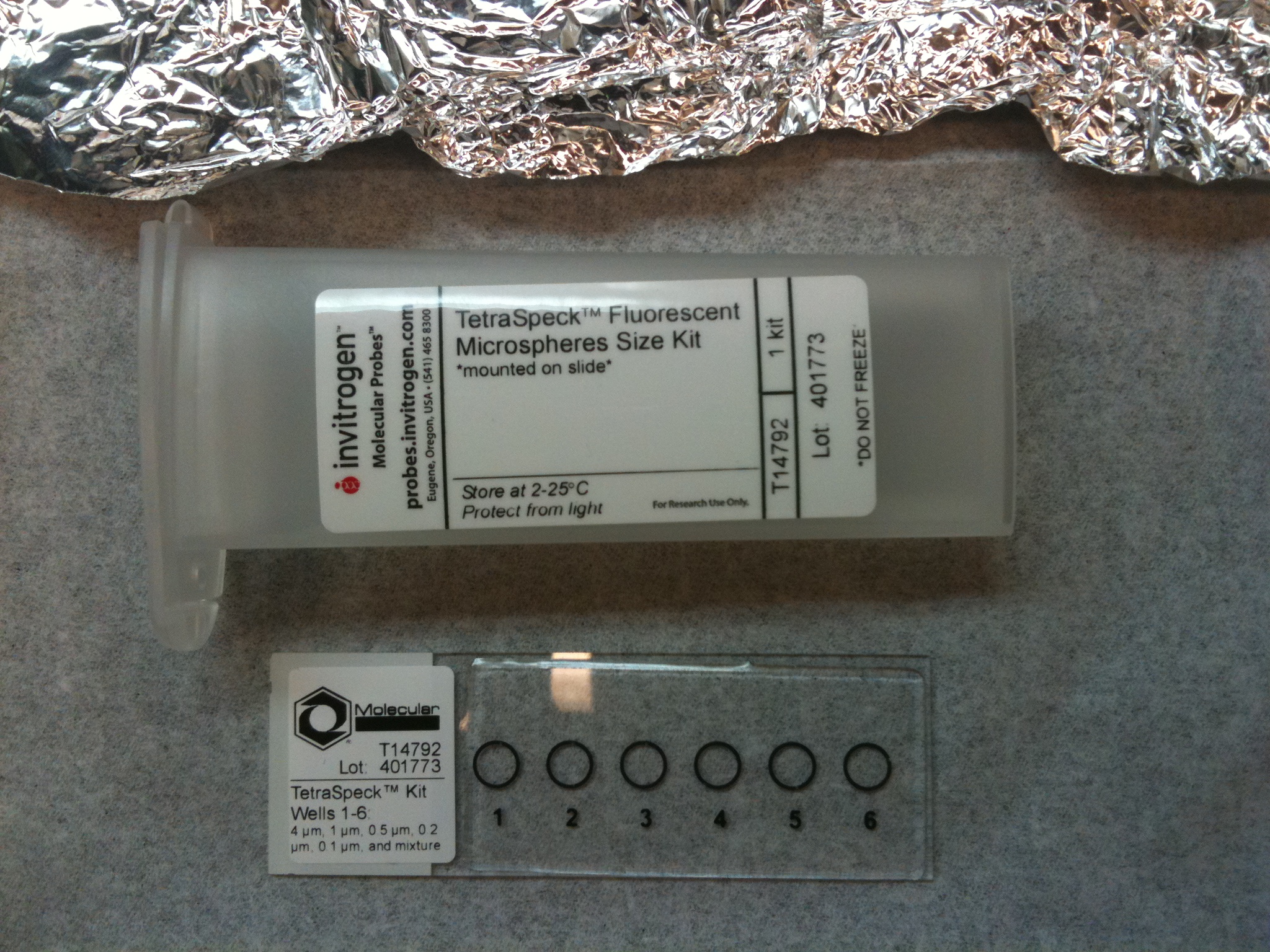
- Fluorescent bead slide
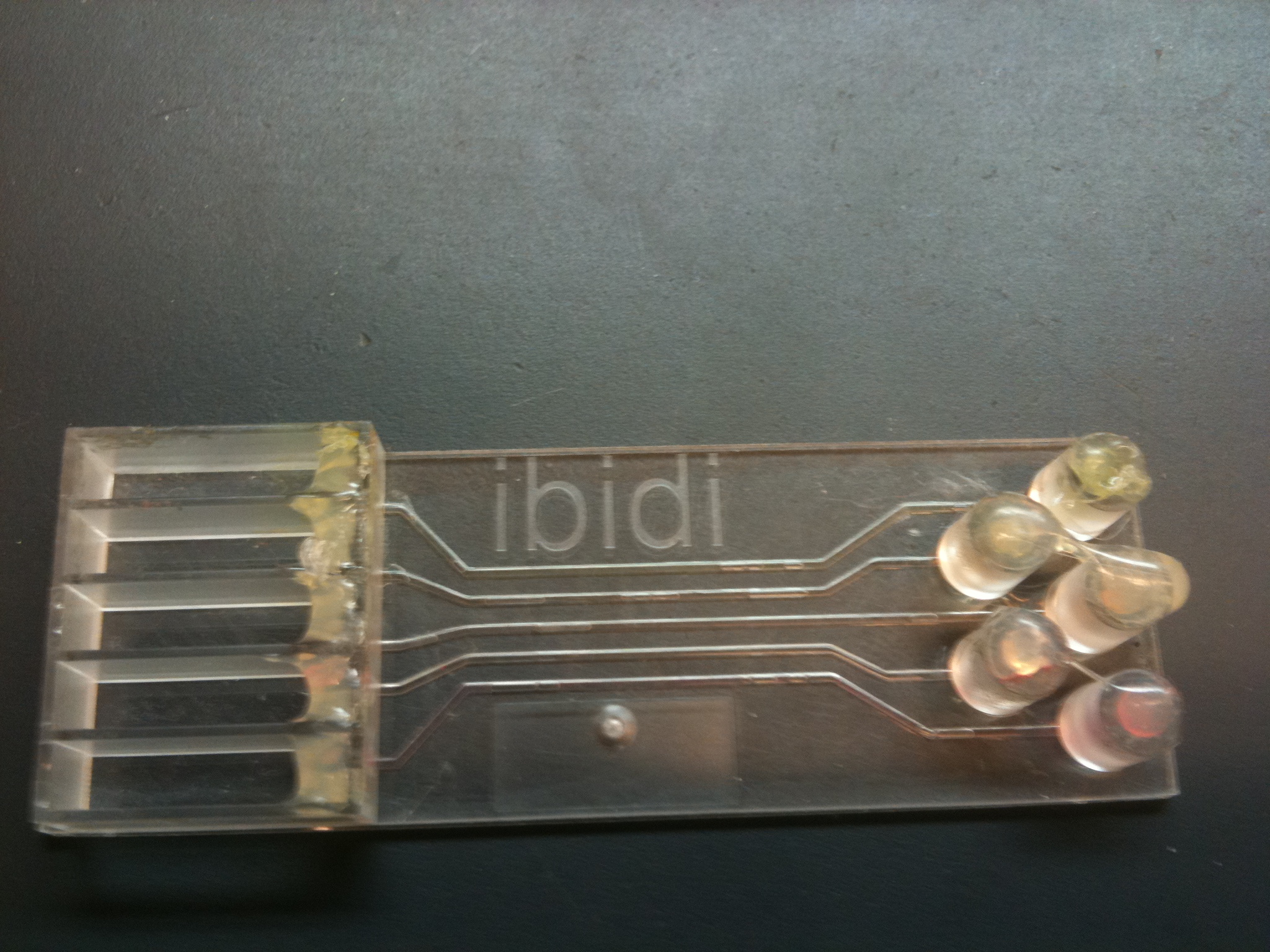
- Fluorescent microchannel slide
- Fresh onion
- Knife and tweezers
- Toothpick or popsicle sticks
- Blank slides and coverslips
- Syringe of vaseline with pipette tip end
- Distilled water
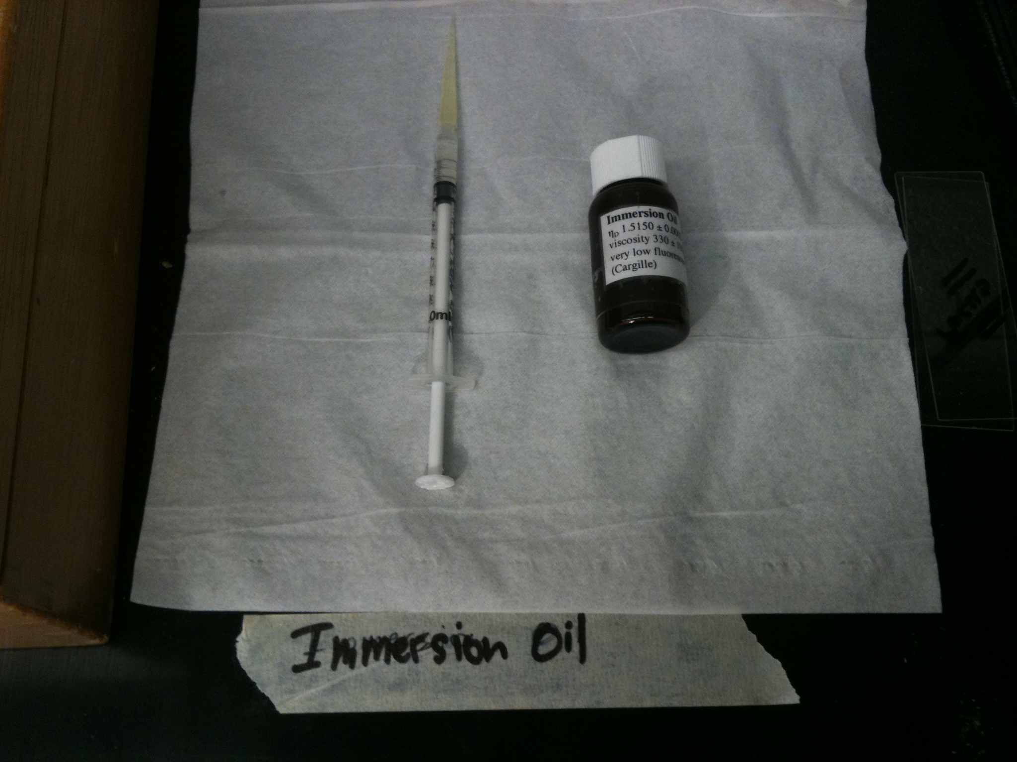
- Immersion oil
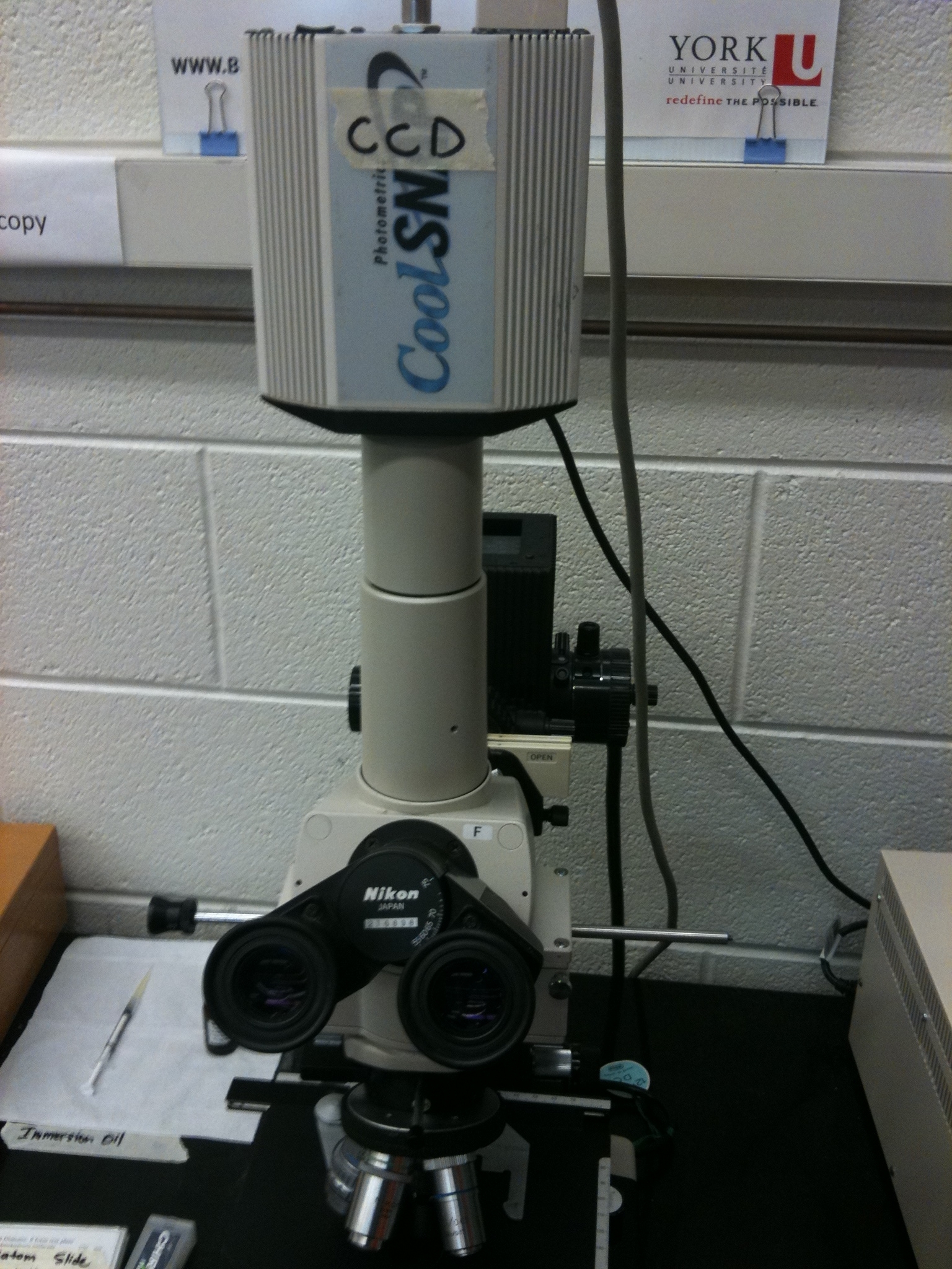
- Nikon upright microscope and CCD camera
- Usb stick for transferring data and images for processing and report generation
Objectives
In this lab students will expand their use of optical microscopes to include fluorescence imaging, which allows for highly specific labelling of proteins and complexes within the specimen. Fluorescence is often complimented with Differential Interference Contrast imaging (DIC), and this will also be explored during these experiments. Fluorescence really is a quantum mechanical phenomenon, and the emphasis here will be on understanding what is physically happening within samples that are fluorescently labelled. Understanding the principle of fluorescence filtering and getting a feel for the light intensity levels being generated is critical for fluorescence microscopy.
Introduction
Fluorescence microscopy is a very powerful tool allowing for the observation and quantification of biological samples. You have seen previous labs how unstained samples contain very little contrast, and through the addition of light absorbing dyes and stains or special optics, the morphology and structure of samples can be readily observed. Fluorescence microscopy uses the same concept of imparting artificial contrast to samples, but has several advantages over absorption based contrast methods. In this contrast method, fluorescent molecules are attached to specific structures within the specimen. Illuminating the specimen with a specific wavelength of light causes these fluorescent molecules to convert some of this illumination into a longer wavelength of light, which is then detected by a CCD or observed directly with the eye.
Fluorescence is a phenomenon first discovered by British scientist Sir George Stokes in 1852. The process involves the absorption of an incident photon of light by a molecule, referred to as a fluorophore, and subsequent emission of a second fluorescent photon a short time later (Figure 1). The energy transferred to the fluorophore after absorption causes the molecule to enter an excited energy state that is short-lived, typically on the order of 10-9 seconds (1/e value). During this time, some of the incident energy is lost due to vibrational/rotational motion and heat, among other things. When the molecule returns to the ground state, a fluorescence photon is emitted at a longer wavelength (lower energy). This fluorescence can be detected with a colour filter that passes the fluorescence emission and blocks the shorter wavelength excitation light. The difference in wavelength between the incident and outgoing photons is referred to as the Stoke’s Shift, and its phenomenon is the basis for all fluorescence imaging as it allows us to use a colour filter set to separate the excitation and emission photons.
 Figure 1 –Schematic representation of the process of fluorescence. Light absorbed by a molecule causes it to move
into an electronic excited state. After losing some energy to heat/vibration/rotation, a fluorescent photon is
emitted and the system returns to the ground state.
|
Fluorescent samples can be stained using two methods; dyes or antibody-based labels. Dyes such as 4’-6’-Diamidino-2-phenylindole (DAPI) or Hoescht are commonly used in fluorescence microscopy to stain nuclei. Both can be used on live or fixed cells, and are relatively inexpensive. Upon incubation with a sample, DAPI binds with A-T rich repeats of chromosomes in the DNA and the fluorescence emission efficiency increases versus its unbound state. This enables visualization of cell nuclei when excited in the ultra-violet (UV) wavelength range and produces blue fluorescent light. The chemical structure as well as absorption and emission spectrum from DAPI are shown in Figure 2.
 Figure 2 –Chemical structure and excitation/emission spectra of DAPI when bound to DNA. DAPI is excited by UV
light and produces blue fluorescent light. Its emission spectrum is quite broad in contrast to other fluorophores.
|
To generate and detect the light emitted by fluorescent molecules some modifications to the microscope light path are necessary (Figure 3). The excitation light is passed through an excitation filter, which reduces the light to a specific wavelength, and is reflected off a dichroic beamsplitter (DBS). A DBS is coated with a special surface designed to reflect light of one wavelength range and transmit a different wavelength range. In the example shown in the figure, the DBS will act as a mirror to blue light, and allow longer wavelength green light generated at the sample to pass through it. The light then passes through one additional filter (emission filter), which further separates any fluorescence from excitation light that may have passed through the DBS.
 Figure 3 - Illumination path in an epi-fluorescence microscope. A filter cube contains an excitation filter, dichroic
beamsplitter, and emission filter and is responsible for separating the excitation light from the generated
fluorescence.
|
The excitation and emission filters as well as DBS are contained within what is called a filter cube, and these can be easily switched while working with the microscope to observe different fluorophores. The microscope you will be working on has space for two separate filter cubes operated on sliders. Other microscopes may use a wheel to translate the filters in and out of the optical path. In highly automated microscopes these filter changes can be motorized and controlled from the microscope software. The DBS directs light at the sample through epiillumination, which means that the objective lens is used to deliver light to the sample and collect the fluorescence emission. Recall that in transmitted light or brightfield imaging, a condenser is used to illuminate the sample from the opposite side of the sample. Using epiillumination to deliver excitation light through the sample allows for more efficient transfer of excitation light to the sample (always a critical concern in fluorescence) and reduces the amount of excitation light re-collected by the objective lens.
A typical configuration for a filter cube optimized for excitation and detection of DAPI is shown in Figure 4 along with the excitation/emission spectra of DAPI. The excitation filter (blue line) transmits light of a specific wavelength range which is efficient at exciting bound DAPI (blue solid area). The DBS (green line) is designed to transmit wavelengths above ~ 410 nm, and thus it will reflect almost all of the excitation light at the sample. The emission filter (red) is used to clean up the light that is collected by the objective and passed through the DBS, and it is optimized for detection of the emission peak of DAPI (red solid area). The emission filters used in your microscope are longpass filters, which are slightly different from the bandpass filter shown below. A longpass filter has a transmission spectrum similar to the tail of the DBS spectra and passes all wavelengths above a certain threshold. This allows for collection of more of the fluorescence signal which typically increases image quality, but prevents multiple fluorophores from being imaged simultaneously.
 Figure 4 - Typical filter cube configuration for detection of DAPI in stained specimens. The bandpass emission filter
(red line) can also be swapped out for a longpass filter, similar in shape to the tail of the DBS spectrum (green line).
|
It is possible to use a single filter cube to visualize multiple fluorophores simultaneously, and while this is often done, it is generally better to acquire fluorescence images one channel at a time. A filter configuration for observation of a common set of fluorophores (DAPI/FITC/Texas Red) is shown below in Figure 5. Note that the absorption and emission maxima have been normalized in the plots below. The relative strength of fluorescence from fluorophores will vary from channel to channel, which will typically require adjustment of the excitation light intensity or CCD exposure time for different channels.
 Figure 4 - Triple filter configuration for detection of fluorophores simultaneously. Bleedthrough of DAPI
fluorescence into the green FITC detection channel often requires images to be acquired individually. FITC and
Texas Red emissions are separated enough to be viewed simultaneously.
|
Shown in the figure are the excitation (dashed lines) and emission (solid lines) of DAPI (blue), FITC (green) and Texas Red (red). To attempt viewing these three fluorophores simultaneously a filter cube would have an excitation filter that passes light in the purple (365 – 395 nm), cyan (475 – 495 nm) and yellow (550 – 570 nm) wavelength regions. These bands are selected to match up with the absorption spectra of the three dyes to be excited. This excitation light would then reflect off of a broadband beamsplitter which reflects only 10-20% of the excitation light to the sample. This is done to maximize the transmission of fluorescence photons back through the filter cube as 80-90% of them will pass through the beamsplitter to be detected. To separate the fluorescence emissions from each other, the emission filter would only pass light in the blue (430 – 460 nm), green (503 – 538 nm) and red (600 – 640 nm) ranges. These ranges are selected to overlap with the fluorescence emissions, and avoid detection of any reflected excitation light collected by the objective lens. To help you visualize the light path a bit better refer to Figure 6 below.
 Figure 6– Triple excitation and emission light path in a fluorescence microscope. The dichroic mirror in this instance is a broadband mirror with 10-20% reflection and 80-90% transmission to maximize fluorescence detection efficiency. The portions of the excitation and emission spectra from DAPI/FITC/Texas Red contained in the filter bandpasses are shown as dashed and solid lines, respectively.
|
On the excitation side we can see that the DAPI excitation actually causes some excitation of the FITC fluorophore. This can cause ghost images to appear if filtering is not properly performed. On the emission filter side we can see that there is no FITC emission in the DAPI detection channel (blue region), and thus the excitation of FITC by the DAPI excitation light is not detected. When examining the FITC emission channel however you can see that there is a significant amount of DAPI fluorescence (blue solid line) that would be passed by the FITC emission filter (green region). This is often a reason why individual excitation and emission filters are used; this issue goes away if no UV excitation light is striking the sample while observing FITC. In contrast, the distance between FITC emission (green line) and Texas Red emission (red line) is large enough that there is a minimal amount of FITC emission passing into the Texas Red detection channel (red region). The take-home message here is that simultaneous imaging can be performed more reliably when the emission spectra are better separated.
Antibody Labelling
While stains such as DAPI will bind to DNA, it stains the whole DNA strand rather non-specifically. Antibody labelling is another way to get fluorescent molecules coupled to the sample, and can be used to identify specific extracellular and intracellular proteins as well as specific mutations or activation regions within DNA. Different cell types express different antigens on their cell surfaces, and antibodies targeted against these antigens allow these cells to be distinguished from each other. While fluorescent molecules such as DAPI stain DNA fragments and yield morphological information on the specimen, the staining is more passive in that all DNA and some RNA is stained. Antibody labelling can be specific to sub-populations of cells or even highly specific regions of DNA. This imparts the ability to visualize the sub-cellular distribution of a wide range of biomolecules and investigate their functions at a molecular level.
 Figure 7– Representation of a 2-step antibody labelling process. A primary antibody is first incubated with the
sample and labels the antigen of interest (left). In a second step, a fluorescent antibody recognizing the primary
antibody labels the cell (middle). After washing any unbound labels, fluorescence from the bound fluorescent
antibody can be detected and quantified (right).
|
Figure 7 demonstrates the concept of fluorescent antibody labelling using a two-stage process (secondary labelling). First, an antibody that is specific to a particular antigen expressed on a cell is incubated with the specimen and binds to the target (left). The power of antibody labelling lies in the fact that the shape of the antibody can only fit with its unique antigen, thus after incubation and rinsing any unbound molecules are washed away. Next, a secondary antibody linked to a fluorescent molecule is incubated with the sample and allowed to bind to the primary antibody (middle). After rinsing and washing again the only fluorescent molecules remaining in the sample are those attached to the target antigen through the antibody link. Excitation/detection can then proceed by using the appropriate filter cube to visualize the localization of the fluorescence signals.
Since multiple biomarkers can be localized in a single specimen through the use of secondary antibodies that excite/emit at different wavelengths (taking cross-talk into consideration as discussed above) fluorescence labelling is a really powerful tool for cell biology. This is because in transmitted light imaging typically one or two labels can be applied to each slide, but with fluorescence imaging the number of fluorescent probes (and thus antigens/proteins studied in the same population of cells) can be significantly larger. A table of common fluorophores along with their excitation/emission wavelengths are shown in the table below.

|
Photobleaching
In general, the fluorescence intensity emitted by a stained specimen is linearly related to the light intensity used to excite the fluorescence. However, there are also probes available that alter their fluorescence quantum efficiency or emission spectra based on the micro-environment they are in. You will not be working with these types of probes in this lab as their use is too advanced for the limited timeframe we have, but it is good to be aware they exist.
The process of fluorescence is inherently destructive to the probe molecules, and there is a limit to how much light a given fluorophore can emit before it loses its ability to fluoresce. This process is called photobleaching, and is generally the result when too much excitation power is placed on the specimen or observation continues over extended periods of time. When this occurs, the fluorescent molecules undergo a structural change which alters their ability to produce more fluorescent photons. Instead, any energy absorbed by photo-destroyed fluorophores is dissipated in a non-radiative fashion. A typical example of photobleaching is shown in Figure 8.
 Figure 8– Example of photobleaching as a function of exposure for a fibroblast cell. Over very long exposures
simulating prolonged observation, the nuclear fluorescence has gone away, and the green fluorescence has faded.
The red fluorescence is virtually unchanged.
|
The specimen is a fibroblast cell, fluorescently labelled with three probe-antibody combinations; Hoechst 33258 (stains nuclei, excited by UV light, produces blue fluorescence), Alexa 488-phalloidin (excited by blue light, produces green fluorescence), and MitoTracker Red (stains mitochondria and cytoskeleton, excited by green light, produces red fluorescence). Images were acquired at 2-min intervals, and the level of fluorescence from the nuclear Hoechst stain can be seen to drop rapidly with exposure to the excitation light, while the signal from the Alexa 488 fluorophore drops only slightly, and the red fluorescence remains constant. Photobleaching complicates the routine use of fluorescence for quantitative studies, and care must be taken to minimize its effects. Often this involves minimizing the excitation intensity of light on the sample and detecting the fluorescence as efficiently as possible. Typically, fluorescently labelled specimens are imaged in a dark environment and are stored in a fridge or freezer protected from ambient light so their fluorescent properties are maintained. It is also very good practice to only illuminate the specimen when collecting data or observing the specimen through the oculars, then close the excitation shutter while saving data and making notes in your lab book (do not turn the lamp on and off however, as this can damage the bulb).
Fluorescence Photon Efficiency
A useful exercise to understand some of the finer points of fluorescence microscopy is to go through an estimation of the generation and detection of fluorescent light from a uniformly fluorescing sample. The excitation source is assumed, for this exercise, to be a standard 75 W xenon arc-discharge lamp having a mean luminous flux density of approximately 400 cd/mm2. When an excitation filter is used to pass blue light from 485 – 495 nm, about 2 mW of light will pass through to be directed at the sample by the DBS in the filter cube (assuming 75% transmission efficiency of the filter). Assume the DBS reflects 90% of this light towards the sample, and that gives a value of approximately 1.8 mW entering the rear aperture of the microscope objective as the excitation beam.
With a 100x/1.4 NA oil immersion objective the area of the specimen illuminated will be approximately 40 μm in diameter, giving an illumination area of 12 x 10-6 cm2. The light flux on the specimen is then about 150 W/cm2, which corresponds to a flux density of 3.6 x 10²⁰ photons/cm2. This illumination intensity on the specimen is about 1000 times higher than that incident on the Earth's surface on a sunny day, yet with all this power only a fraction will generate fluorescence that is collected, passed by the optical filters and detected by your eye or the CCD camera.
The fluorescence emission that results from the light flux discussed above depends on the absorption and emission characteristics of the fluorophore, its concentration in the specimen, and the optical path length of the specimen. We are considering a uniformly fluorescing material, and in mathematical terms the fluorescence produced (F) is given by the equation:
|
|
Where σ is the molecular absorption cross-section, Q is the quantum yield, and I is the incident light flux (estimated above to be 3.6 x 10²⁰ photons/cm2). Assuming that FITC is the fluorophore being excited, σ = 3 x 10-16 cm2/molecule, Q = 0.99, resulting in a value for F of 100,000 photons/sec/molecule. If the dye concentration is 1 μM/L and is uniformly distributed in a 40- micrometer diameter disk with a thickness of 10 μm (volume = 12 pL), there will be approximately 1.2 x 10⁻¹⁷ moles (7.2 million molecules) in the optical path. If all of the molecules were excited simultaneously with a bright pulse of light, the fluorescence emission rate will be:
|
|
The question of interest is how many of the emitted photons would be detected and for how long could this emission rate continue? The efficiency of detection is mainly a function of the optical collection efficiency (lens NA plus associated losses from filter cubes) and detector quantum efficiency. A 1.4-numerical aperture objective with 100% transmission (an unrealistic condition) has a collection efficiency of about 30%, which is actually quite high considering a lens with a 90 degree collection volume (again, an unrealistic condition) would only collect 50% of the generated fluorescence. The transmission efficiency of the DBS is typically 85% and the emission filter will typically pass 80% of the in-band light. The overall collection efficiency is therefore about 20%, or 1.4 x 10¹¹ photons/sec. If the CCD has a typical sensitivity, the quantum efficiency is about 50% for the green FITC emission (at 525 nm), so the detected signal would be 7 x 10¹⁰ photons/sec. Comparing this value to the fluorescence emission rate calculated above shows that only 10% of the generated fluorescence actually contributes to the signal you are seeing. Even with a perfect detector (again, an unrealistic assumption), only about 20% percent of the fluorescence emission photons can be detected. If an objective with a lower NA is used (the 100x used in this example has a very high NA), the detection efficiency again drops further.
Another important note to re-iterate here is the effect of photobleaching. For FITC in an oxygenated saline solution each molecule can only emit about 36,000 photons before being destroyed. In a deoxygenated environment, the rate of photodestruction diminishes about tenfold, so approximately 360,000 photons/molecule can be produced. The entire volume of fluorophores in our uniform sample contained 7.2 million molecules. Therefore, a minimum of 2.6 x 10¹¹ and a maximum of 2.6 x 10¹² fluorescence photons could be produced before photobleaching starts to diminish the signal noticeably. Assuming the emission rate of 1 x10⁵ photons/sec/molecule calculated above, fluorescence could continue for only 0.3 to 3 seconds before photodestruction begins. In the case where 10% of the photon flux is detected, a signal of 7.2 x 10¹⁰ photo-electrons/second would be obtained at the CCD detector.
The numbers above certainly convey that fluorescence imaging is inherently performed under low-light imaging conditions, and care must be taken to reduce background and stray light from being detected and washing out the fluorescence signal. Following the argument of this example, if the CCD contains a 1000 x 1000 pixel array, this signal would be distributed over a million pixels, or approximately 72,000 photo-electrons per sensor. For a CCD with 9 μm2 pixels the storage capacity is about 80,000 photo-electrons and the read-out noise is less than 10 electrons. The signal-to-noise ratio would then be largely determined by photon statistical noise:
|
|
In almost all cases, this high signal level could only continue for a very brief period of time before photodestruction occurs, and it is ultimately impractical to run with excitation powers high enough to photobleach this quickly, especially in live cell fluorescence imaging. The compromise utilized by most microscopists to prolong the observation period is a 10-20x reduction in the excitation light intensity so that only a fraction of the fluorophore molecules are excited and subjected to photodestruction at a given time. Thus, the signal-to-noise ratio rarely equals the theoretical maximum in this example, and typically ranges between 10 and 20 in fluorescence microscopy.
One final note of caution with fluorescence microscopes has to do with proper care of the excitation lamp. These light sources need 5-10 minutes to warm up and become stable before they should be used. After turning on the power wait 5 minutes before pressing the second push button on the power supply. Once you have turned the fluorescence lamp on, it should be left on for the duration of the lab, and you should use the shutter to control when light reaches the sample for imaging.
DIC Imaging
The image forming physics and optical light path in DIC microscopy are quite different from modes explored so far in these labs, and has the most in common with phase contrast imaging in that both techniques enhance visualization of the optical path of samples. Recall that in a phase contrast microscope optical path length changes create phase delays in light passing through transparent samples, and interference is used to translate these phase changes into visible intensity changes. In DIC imaging, optical path length gradients (in effect, the rate of change of the optical path length) are primarily responsible for contrast. Steep gradients in path length generate excellent contrast, and images display a pseudo three-dimensional relief shading, which is characteristic of the DIC technique. Regions having very shallow optical path slopes, such as those observed in extended, flat specimens, produce insignificant contrast and often appear in the image at the same intensity level as the background. DIC works on the principle of interferometry to gain information about the optical density of the sample. A relatively complex lighting scheme produces an image with the object appearing black to white on a grey background. This image is similar in appearance to that obtained by DPC microscopy but without the bright diffraction halo around areas where the index of refraction changes. DIC is often used in combination with fluorescence samples to add morphological context to fluorescence images (see Figure 9).
 Figure 9– DIC and fluorescence images of two cell types. Both cell types are visible in the DIC image. Only fluorescing cells are present in the fluorophore image.
|
DIC works by separating a polarized light wavefront into two orthogonally polarized mutually coherent parts which are spatially displaced (or sheared) at the sample plane by a Wollaston prism (Figure 10). A Wollaston prism consists of two calcite prisms cut at right angles and mounted so that their optic axes are perpendicular to one another. The direction in which the polarizations are separated is called the shear direction. The outgoing light beams diverge from the prism yielding two polarized rays, with the angle of divergence determined by the prisms' wedge angle and the wavelength of the light. The displacement between these two polarizations is exaggerated in the figure, typically it is much less than the resolution limit of the microscope on the sample (i.e., < 0.2 μm).
 Figure 10 -Optical path through a DIC microscope. Light is split into two orthogonal polarizations by a Wollaston prism and focused onto the sample. A second Wollaston prism recombines the two beams so they can interfere and produce the DIC effect.
|
After passing through the sample and being collected by the objective, these two polarized wavefronts enter a second Wollaston prism which recombines them, causing them to interfere with one another. If each of these wavefronts were observed individually before recombining, they would each have the appearance of a brightfield image, i.e. only intensity variations due to absorption would be visible. These two images do not quite line up because of the illumination shear introduced by the first Wollaston prism. This means that instead of interference occurring between rays of light that passed through the same point in the specimen, interference occurs between rays of light that went through adjacent points which therefore have a slightly different optical path. This recombination of light causes "optical differentiation" of the optical path length.
The second Wollaston prism is also used to vary the phase bias offset between the two polarizations. This is accomplished by translating the prism, changing the relative path lengths through each of the calcite wedges. The effect of this in the final image is to go from a darkfield type image, where most of the light is destructively interfered, and results in a pseuso three dimensional, which is image typically associate with the DIC mode. In both of these images, the features you see are not due to absorption differences in the sample, nor are they topographically representative of how the sample actually ‘looks’ to your naked eye since much of the contrast is generated by optical path differences you cannot typically see.
Since DIC contrast depends in some part to preserving the polarization of the light waves interacting with the sample, the use of plastic slides or culture dishes can destroy the contrast of the sample since plastic destroys this polarization relationship between wavefronts. This is not an issue for phase contrast imaging. One disadvantage of phase contrast imaging in combination with fluorescence is that the phase ring etched into the objective actually blocks some of the light collected by the lens which reduces light collection efficiency when used for fluorescence collection. DIC objectives do not have this limitation, and for this reason it is typically this mode that is used in conjunction with fluorescence imaging where we have just seen how efficient photon detection is very important.
As with phase contrast imaging, there is a procedure you must follow for proper alignment of the DIC optics. Refer to Appendix 1 for this procedure.
Methods
A schematic of the microscope you will be using in this lab is shown in Figure 11. You can use this figure as a reference when performing the alignment and configuration of the microscope during the lab. Of particular note is to make sure you have the correct condenser fitted on the scope for this lab, which is the DIC. When imaging in fluorescence it is good practice to turn off the room lights. This will help reduce detection of scattered light as well as dark-adapt your eyes to make the low level fluorescence signals easier to see visually. Find the location of the mercury light shutter and slider bars for moving the fluorescence filter cubes in and out of the optical path, and be sure to keep the shutter closed and only open it for brief periods during fluorescence imaging.
 Figure 11 -Schematic of the Nikon microscope you will be using in this lab. Refer to this figure to familiarize yourself with the components and their locations.
|
Alignment of the DIC transmission optics is covered in Appendix 1, and initially you will look at transparent cheek epithelial cells, which you worked with in the previous lab, and move on to fluorescently labelled samples. If you have time at the end of the lab and are interested you can switch back to the phase contrast condenser and come back to the samples to compare DIC and phase contrast. When working with DIC and fluorescence it is important to remember to remove the polarizer from above the objective as well as the Wollaston prism when switching from DIC to fluorescence, otherwise the fluorescent signal will be attenuated further and your image exposure times will be extremely long.
The first fluorescent samples you will look at are made up of polystyrene microbeads (0.02 – 4 μm in diameter) which have been infused with a mixture of fluorescent molecules. Samples such as these are often used as resolution and intensity standards for fluorescence measurement devices. One slide contains microchannels which contain mixtures of two fluorescent microbeads too small to be resolved optically (0.02 μm) in diameter, so the bead solution appears like a homogeneous fluorescing medium like the example discussed above. Using this slide you will see how different wavelengths of light excite each fluorophore, as well as using time-lapse imaging to observe photobleaching in action. The second microbead slide consists of a series of circular areas which contain different sized microbeads in mixtures and on their own. The diameter decreases from 4 μm beads down to 0.02 μm, in the first five areas and in area number six there is a mixture of all sizes. Using this slide as well as spatially calibrated images you will measure and verify the size of the microbeads. Since these fluorescent beads are designed for routine calibration and testing of fluorescence systems, they are less susceptible to photobleaching than stained slides. That being said, care should still be taken to store these slides in the dark and try to limit the amount of light exposure they receive so that they last longer.
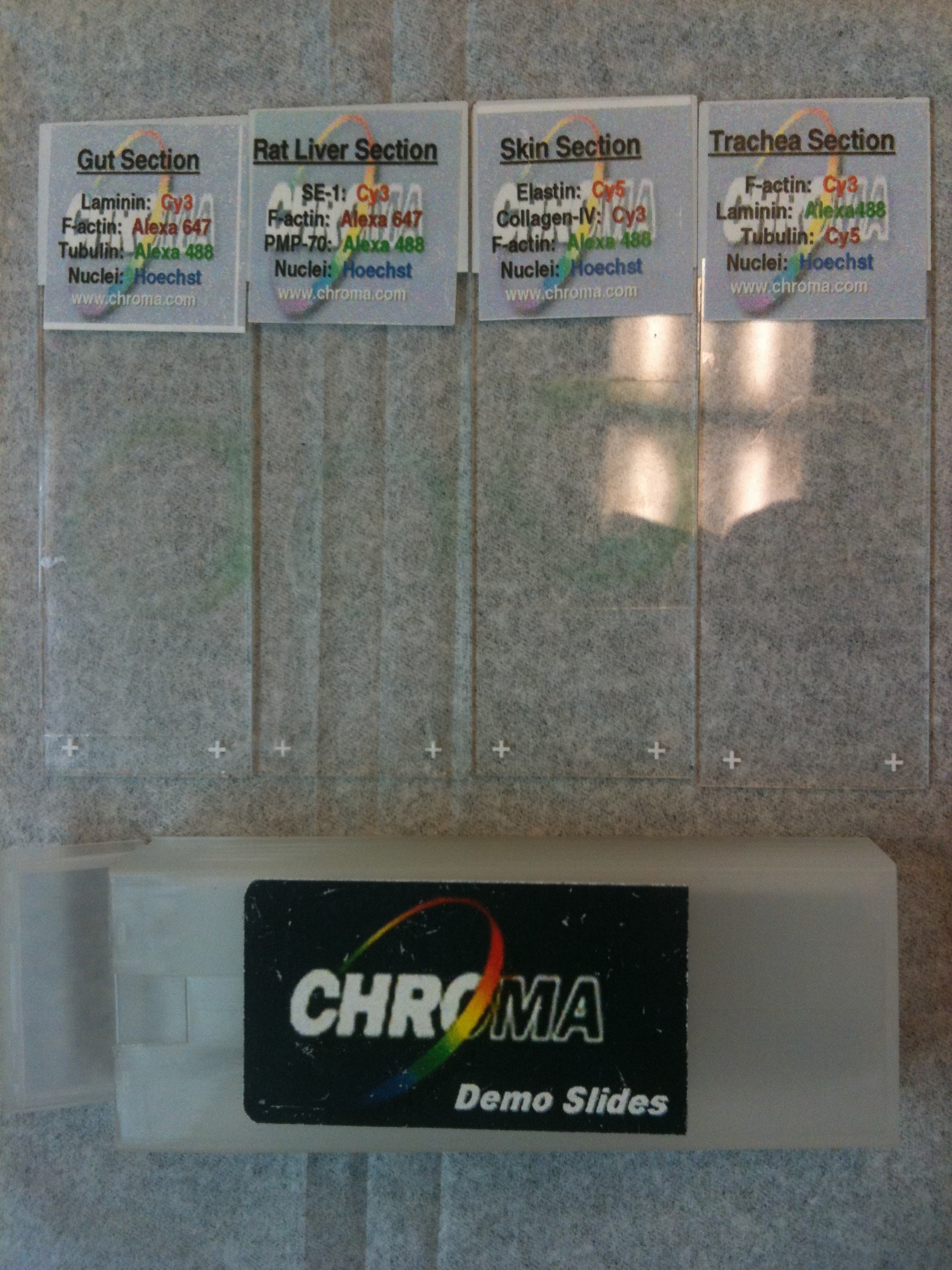
The fluorescence tissue sections used are from a set of four fluorescently labelled slides designed to act as a reference standard for microscope performance. They are optimized for measuring specific performance parameters of instruments, including resolution, cube performance or spectral separation and camera sensitivity. All four slides are labelled with the same fluorophores: Hoechst (UV excitation, blue fluorescence), Alexa488 (blue excitation, green fluorescence), Cy3 (green excitation, orange/red fluorescence) and Cy5 (red excitation, far red/IR fluorescence). The microscope you are using does not have a filter for the Cy5 dye, however, red excited dyes like Cy5 are difficult to visualize in any case because the human eye’s sensitivity to light past 700 nm is very poor. CCD detectors, on the other hand, are sensitive well into the IR and with the proper filter set digital images of Cy5 are efficiently captured.
One major advantage of dyes in the red excitation regime is that they excite less tissue autofluorescence, which can be problematic for UV, blue and even green excitation wavelengths. Tissue autofluorescence is the term used to describe background autofluorescence from the tissue specimen itself. There are a number of compounds naturally present in specimens which fluoresce naturally in live as well as fixed tissues. Tissue processing and fixation is also known to increase tissue autofluorescence, and the end result is often the reduction (and sometimes inability) to detect the fluorescence from the antibody or dye label which has been added to the specimen. Tissue autofluorescence from live cells originate from the mitochondria and lysosomes, most specifically from coenzymes such as nicotinamide adenine dinucleotide (NADH) and flavins such as flavin adenine dinucleotide (FAD). The fluorescence produced by these compounds have very broad emission spectra that can overlap much of the visible spectrum, making it almost impossible to eliminate their influence in fluorescence images with traditional filtering methods. In live tissues, collagen and elastin contribute greatly to autofluorescence, and generally express more endogenous fluorescence than cells in culture. The set of four fluorescent slides all exhibit moderate amounts of autofluorescence, and are sections of rat liver, skin, gut (ileum) and pancreas.
The liver, after the skin, is the largest organ in the body and its job is to process a huge variety of nutrients for use by individual cells throughout the body. The primary cell type within the liver is the hepatocyte, which is responsible for protein synthesis and storage as well as detoxification. Nuclei are stained with Hoechst, peroxisomes are stained with Alexa488, sinusoidal endothelial cells are stained with Cy3, and actin filaments are stained with Cy5. The key labelling components of this slide are the peroxisomes. Peroxisomes are organelles present in almost all eukaryotic cells and contain enzymes which rid the cell of toxic peroxides. They are bound by a single membrane which separates their contents from the cytosol (the internal fluid of the cell) (Figure 12). Each peroxisome is labelled with a primary antibody to PMP 70 which is linked to Alexa488. This molecule is abundant in the membrane layer. The size of individual peroxisomes varies between about 200 – 400 nm in cross section, as such they can be used as a resolution standard for light microscopy. If you examine the slide using a high NA objective (oil 40x or oil 100x) it should be possible to see the peroxisomes as “donuts” within the cell, at lower NA they appear as round solid structures.
 Figure 12 -Basic structure of a peroxisome. With fluorescent membrane staining and high resolution optics they appear as donut shaped objects in fluorescence images. Autofluorescence and photobleaching can make them difficult to detect.
|
The skin section is stained with Hoechst for nuclei, Alexa488 for actin, Cy3 for elastin, and Cy5 for collagen. The skin is the largest organ in the body; it cushions the body from assault, is the primary surface for heat regulation, and is a primary sensory surface. In this section the most obvious cellular structure is the stratum corneum (surface of the skin) and constitutes the top ten or so cell layers visible in the section. Immediately beneath the epidermis is a thin though tightly defined layer of basement membrane, labelled with antibodies to collagen IV. This thin layer essentially separates the epidermis from the dermis. The dermis has a rich blood supply and constitutes the “elastic” part of the skin. This tissue was chosen as it represents one of the more difficult structures in the body to image; apart from the principal cellular structures defined above you should also see significant autofluorescence from the elastin. This is particularly evident when using excitation from the UV through blue excitation. In fact it is reasonable to use autofluorescence to collect a useful image of the elastin in skin or large blood vessels.
The gut section is stained with Hoechst for nuclei, Alexa488 for tubulin, Cy3 for laminin and Cy5 for actin. The gut is one of the primary absorptive surfaces in the body, and is made up of tiny folds of tissue called villi. Villi look like ‘fingers’ and line the interior wall of the gut, and their shape serves to increase the surface area of the interior wall. The apex of each epithelial cell in villi is covered with actin rich microvilli, about 400 nm long that should be easily defined with any high NA objective above 40X. Goblet cells which intersperse the epithelial cells can be seen to be full of mucus droplets, and appear as vacuoles under H&E staining (Figure 13). This is an excellent slide to use in conjunction with DIC as the droplets are not visible in the fluorescence images, and easily seen in DIC. Under the epithelium is the lamina propria, which is highly vascularised tissue lining the gastrointestinal tract.
 Figure 13 – H&E stained villi in a gut section. The large surface area of the villi is comprised of epithelial cells which contain tiny microvilli on their interior surface (not visible in figure), as well as goblet cells, which are primarily responsible for mucus secretion and storage (arrow).
|
The pancreas is important for producing several hormones in the body, such as insulin, and enzymes which aid in the breakdown of carbohydrates, proteins and fats. The pancreas section is stained with Hoechst for nuclei, Alexa488 for actin, Cy3 for insulin, and Cy5 for laminin. Individual pancreatic islets are stained for insulin to highlight the beta cells. These structures, like the peroxisomes in the liver sample, should be visible as discrete structures at high NA. However, unlike the peroxisomes, the beta cell granules are stained throughout and do not appear hollow.
Experiments
Before beginning the experiments there is one useful tip in working with fluorescence images which you may find useful: false-colouring the image from the CCD displayed on the computer monitor. This feature changes the image displayed from a greyscale image into a colour palate selectable from within the Image -> Lookup Tables menu in ImageJ. This will match the fluorescence emission colours you see with your eye (to a certain extent) and make the digital image more pleasing to view in some cases. Use blue when looking at DAPI, green when looking at Alexa488 and red for Cy3.

|
Also, when working with fluorescent images acquired with different filter cubes it is sometimes desirable to combine individual images into a colour composite image. For example, if you acquire one image using the blue excitation (producing green fluorescence) and another image using green excitation (producing red fluorescence) it is desirable to produce a colour composite of these two images. For this to work properly care must be taken that the sample is not shifted on the microscope when switching filter cubes or the images will not overlay properly. To overlay images in ImageJ select ‘Merge Channels’ from Image -> Colour:

|
Select the appropriate colour for the merge overlay (UV/DAPI excitation = blue, blue/Alexa488 excitation = green, green/Cy3 excitation = red). If there are only two fluorescence channels, select ‘none’ in the drop down menu. If you are overlaying a DIC image on top of the fluorescence image, select the DIC image as the greyscale overlay. Also, uncheck ‘Create Composite, and check ‘Keep Source Images’ to keep the individual image channels open. When you click ‘OK’, the images will be merged into a colour overlay which you can save.

|
Finally, before getting to the experiments, here are some tips and reminders for working with fluorescence samples and combining the use of fluorescence with DIC imaging:
-
- Ensure the room lights are off when working with fluorescence images. For this lab it would be good to work with the lights off for the duration, and use a small desk lamp for writing notes and seeing what you are doing.
- Be liberal with the shutter controlling whether excitation light is reaching the sample or not and try not to leave the sample exposed to excitation light for more than 5-10 seconds at a time unless you are moving around looking for areas to focus in on.
- Be sure to block the transmitted light or turn the halogen lamp (not the fluorescence lamp) off while acquiring fluorescence images. You can also leave the lamp on and block the light by placing an object underneath the condenser to block light from reaching the sample. This may be easiest.
- Before acquiring fluorescence images make sure to remove the top polarizer and DIC prism from the mount on top of the objectives.
- Likewise, replace the polarizer when acquiring DIC images, also making sure that you remove the fluorescence filter cube from the light path.
- Clean oil objectives and re-useable slides thoroughly when finished. Inspect the lens with one of the eyepieces to verify it is clean.
- Align DIC mode using the method in Appendix 1.
- Prepare another cheek sample and onion sample as you did in the previous lab and observe them in DIC using the 20x and 100x DIC objectives. Be careful not to transfer any oil onto the 20x objective.
- Fluorescence excitation and photobleaching of sub-resolution bead mixtures.
- This sample is quite bright compared to typical fluorescent specimens, and contains beads ideally excited by blue and green light. You will notice that the blue light will actually excite both dyes.
- The microchannels contain mixtures of the two beads in the following ratios: 100:0, 75:25, 50:50, 25:75, 0:100.
- Acquire images of each of five microchannels using blue and green excitation light and the 40x oil objective.
- Set the exposure of the CCD to the value required to see the brightest microchannel without saturation, and use this exposure for all images using this that filter. In other words, you will have two image sets containing five images/set. Each image set should use the same exposure setting.
- Calculate the relative bead mixture ratios from your data set (Note: you can do this part after acquiring the time-series and putting the slide back).
- Open the image sets from the blue and green excitation wavelengths in ImageJ.
- Using the ‘Rectangular Sections’ tool in ImageJ, draw a box within the fluorescent area of the data set.
- Pressing ‘Control + M’ on the keyboard will measure the intensity and standard deviation of the area within the box and input the results into a text box for.
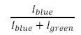
- Using the measured intensity calculate the relative bead abundances in each of the microchannels by taking the intensity of a given microchannel and dividing it by the sum of the intensities from the green and blue excitation wavelengths (see below).
- How do your values compare with the physical amount of beads present in each sample?
- Using the appropriate excitation wavelength and exposure for the channels on the
edges (100:0 & 0:100 mixtures, blue and green excitation) set up a timed acquisition in
μManager (refer to the previous lab if you need a refresher on how to do this) with the
following parameters:
- Number of frames = 100
- Interval = 30 seconds/frame
- Open the time series and create and image stack of the data set and save it (see
previous lab for instructions if you don’t recall how to do this).
- Using the ‘Rectangular Sections’ tool in ImageJ, draw a box within the fluorescent area of the data set that contains a relatively uniform region of fluorescence.
- Pressing ‘Control + M’ on the keyboard will measure the intensity and standard deviation of the area within the box and input the results into a text box for further processing.
- Switch to the next image in the stack by pressing the ‘>’ key, and measure the intensity again by pressing ‘Control + M’.
- Repeat until you have gone through all frames in the stack.
- Save the results file as a text file, import it into a spreadsheet program (Excel is installed on the PC if you wish to do it now, or you can take the files with you and do it at home as well).
- Create a plot of intensity versus time (remember, the frames are 30s apart) for each of the data sets. What do you notice about the intensity as a function of time? Does one of the data sets show a larger effect?
- Liver slide
- Obtain the fluorescent liver slide.
- Using the 20x objective, find some areas with bright staining and move to the 40x (oil) and 100x objectives.
- Try and observe the peroxisomes using the lower resolution objectives (10x/20x). Do you see them as donuts or spots?
- Using the 40x (oil) and 100x objectives acquire fluorescence images using all three filter cubes, particularly focusing on getting good clean images of the peroxisomes, which should look like small ring shaped objects with these objectives.
- Save all images and clean the slide and put it away.
- Peroxisome measurement and RGB image generation.
- Input the spatial calibrations you calculated previously for these objectives and generate and RGB merged image using the method described above.
- Measure the size of the peroxisome, which should be around 200-400 nm. Do your measurements agree?
- Gut slide
- Obtain the fluorescent gut slide.
- Browse around the slide and locate some villi.
- Acquire images using 10x and 20x objectives with all filter cubes as well as by sliding the DIC polarizers and prisms in place and acquiring a DIC image (note: DIC is only possible using the 20x and 100x objectives on this system).
- Repeat with the 100x objectives.
- It may be useful to take the DIC images first to make sure that you see some goblet cells in the field of view on the camera.
- Save all images and clean the slide and put it away.
- Image manipulations in ImageJ.
- Produce a fluorescence/DIC overlay in ImageJ of the frames you acquired using the method described above.
- Using spatially calibrated images, measure the size of the microvilli on the columnar epithelial cells. They should be approximately 400 μm in length, and barely visible on the 100x objective.
- Also measure the diameter of the mucus secretions in the goblet cells.
- Both of the above measurements may be easier to perform on the original greyscale data rather than the colour composite.
- (OPTIONAL) Fluorescence of microbeads
- Obtain the fluorescent microbead slide. There are six regions marked on the slide, the first five contain beads of a single size, and the last contains a mixture of all bead sizes.
- Unlike the previous slide, the beads in this slide are each stained with four fluorophores, and thus will be visible using all filter cubes. These beads will be visible as discreet objects with most of the objectives. Use the filter cube which produces the lowest CCD exposure setting for this slide.
- Acquire images of each of the six areas using the 10x, 20x, 40x (air & oil) & 100x objectives.
- Take DIC images of beads on the area containing the bead mixtures (20x & 100x).
- After you are finished with the slide, clean it using the supplied cleaner and return it to its light protected box.
- Bead size calculation and comparison of NA collection efficiency
- Open the images in ImageJ and calibrate the spatial pixel size using the values you calculated in the previous lab using the calibration slide. You can also recalculate them using the calibration slide again if you don’t have the numbers handy. Follow the procedure in the previous lab if you need to do this.
- Zoom in to a visible bead in an image and using the ‘Elliptical Selection’ tool in ImageJ draw a circle around the bead and press ‘Control + M’ to measure its intensity.
- Use the ‘Straight Line Selection’ tool in ImageJ to measure the diameter of the bead.
- Repeat this for five beads and calculate an average size and average intensity for each of the five bead sizes. Do this for the 40x (air & oil) as well as 100x objective images.
- For the intensity values from the 40x air and 40x oil images, normalize the
intensity by the exposure setting used for each of the images. In other words, if
you used a 100 ms exposure for the 40x oil and 400 ms exposure for the 40x air:
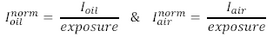
- What do you notice about the normalized intensity between the air and oil objectives? Does this make sense?
- What is the minimum objective required to resolve all of the beads? Does the lens NA play a factor in this at all?
- (OPTIONAL) Skin slide
- Obtain the fluorescent skin slide.
- Switch between filters and objectives while browsing around the slide. Of particular note is to observe how bright the autofluorescence is and how it is present in virtually all image channels. As discussed above most of this autofluorescence is due to elastin within the tissue.
- There is no need to acquire images of this sample, but if you have time and you wish to, you can acquire and generate an RGB overlay using the objectives of your choosing.
- Save all images and clean the slide and put it away.

Questions
- What transmitted light mode is best used with fluorescence and why?
- Describe why using a higher NA lens for fluorescence is advantageous.
- Describe what photobleaching is, and steps that can be taken to minimize it.
- Describe some advantages of fluorescence labelling.
- In the bead slide, what objective performed the best at resolving all beads as well as giving the strongest signal?
- How did your exposure settings vary between the microchannel slide, microbead slide and tissue section slides? Using these values, estimate the relative difference of fluorescence emission rates from each of these samples.
Appendix 1 – DIC Optical Alignment
First, start by making sure that you are using the DIC condenser on the microscope. If not, ask your lab instructor or get it from the wooden condenser box and replace the phase contrast condenser with it.
- 1. The optical path of a DIC microscope and its main components are shown in the figure below. Alongside this figure are actual images of what the components look like when removed from the microscope.
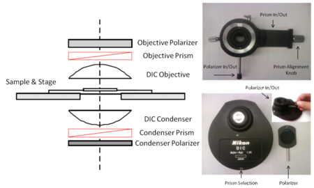
- Using the figures above as a reference, locate the condenser polarizer and prism selection turret, as well as the objective polarizer/prism mount on the microscope. In general you can work with the condenser polarizer always in position. The objective polarizer and prism should be removed from the optical path when performing fluorescence imaging.
- To start, remove the objective polarizer and prism (above the objective) from the optical path by sliding out the pin and prism block on the mount.
- Switch to the 20x DIC objective and focus on an unstained slide (cheek cell, baboon eye, onion cell, etc) sample using regular transmitted light.
- Set the microscope up for Kohler illumination (see the previous lab if you need a refresher).
- At this point you want to align the two polarizers for maximum extinction (maximum darkness) when both are inserted into the optical path. This is also known as ‘crossing the polarisers’ since the maximum extinction condition arises when the transmission axes of the polarisers are orthogonal, or crossed.
- To do this, loosen the mounting pin for the prism assembly above the condenser which is located on the left side of the microscope, silver knob on the microscope frame just above where the prism assembly mounts into the scope. Using both hands slowly rotate the condenser until the minimum amount of light is visible.
- Tighten the stage condenser back to lock it into position.
- Insert the objective prism into the optical path by pushing the slider to the left.
- Now rotate the condenser prism into position for the objective you are using (i.e., ‘20’ for the 20x objective, and if using the 100x objective you would rotate the condenser to the ‘100’ setting).
- Replace the eyepiece and observe your specimen again.
- Turn the prism alignment knob all the way in (turning clockwise). At one extreme you will see the specimen become highly coloured, which is not the alignment you want for traditional DIC.
- Rotating the knob in the opposite direction, you should get to a position (near the middle of travel) at which the specimen exhibits a high degree of contrast, and appears to be illuminated from an oblique angle. Moving a little bit further, you will notice that the direction of illumination apparently changes 180° (ie, from top-left to bottom-right).
- The alignment you want to be at is either side of this central point, and the image should present itself with a pseudo-3D, or embossed, appearance. The specimen should now exhibit a high degree of contrast.
- Double check the Kohler illumination.
- Two final notes:
- The direction of the ‘shadowing’ observed is the sheer angle (the angle between the laterally sheared beam produced by the condenser prism). The distance between an adjacent light and dark spot is the sheer distance, which is typically set to match the resolution of the objective lens being used in green light. This is why you need to use a different condenser prism for the 20x and 100x objectives.
- Finally, remember that the topographic look of the image is not directly related to sample thickness, but the rate of change of optical path length within the specimen.
