Main Page/PHYS 3220/Particle Tracking
Contents
Particle Tracking Chamber Simulation
Onscreen Particle Physics is a software package that is used as a tool to introduce some phenomena and methods of particle physics. Particle production and the subsequent spontaneous decays, and associated lifetimes are some basic concepts. Such decays are constrained by the laws of conservation of momentum and energy. In addition, at high energies, relativistic kinematics will have to be employed. The aim of this simulated tracking device experiment is to understand the process of generation and decay of the following particles: the neutral pion, charged pions and muons.
Introduction
There are three basic parts to the Onscreen Particle Physics program: (1) The Trackmaker is an interactive simulator through which you will learn how different values of the magnetic field or velocity of an incoming particle affect the motion of the particle(s) in the chamber. You should be able to understand the trajectory as a direct result of the Lorentz force. (2) The second part is the particle detection facility, which is a three dimensional chamber that allows projections and rotations of the particle to be observed as it traverses the chamber. The primary particle is allowed to decay, and the charged products of the decay then follow paths specified by their energy and momentum. (3) The third part is a Reminder utility that can be used to remind the student of useful equations, such as the Lorentz force, or the expression for the momentum of a charged particle in a magnetic field perpendicular to its plane of motion.
The Onscreen Particle Physics program allows you to develop an understanding of spontaneous decays. In the microscopic domain, quantum mechanics does not permit us to think of particles as having well defined trajectories. Similarly, for spontaneous decays (cf.. radioactivity) we cannot predict at what moment any single particle will decay. We are only allowed statistical information for an ensemble of particles. ChamberWorks uses a random number generator to simulate decay events according to the known lifetimes of the particles involved. In fact, it even knows about branching ratios (relative probabilities), if particles have different modes of decay.
Spontaneous decays follow an exponential decay law. The lifetime (τ) of a particle is defined as the time at which the number of states or particles surviving is e-1 of the number present initially. In contrast, the half life (τ1/2) is the time at which the number of particles surviving is 1/2 of that present initially, where τ1/2 = (ln 2) τ = 0.693 τ.
Experimental Procedure
Familiarize yourself with the write-up in the Onscreen Particle Physics User's Guide[1]. A quick reading of the manual will help you to get oriented, but you will need to review the material more carefully as you perform the experiment. Prior to starting the experiment, refresh your knowledge of relativistic kinematics, (e.g. the chapter on Relativity in Halliday, Resnick, Walker[2]) and the motion of charged particles in a magnetic field. Understand the units for mass and energy as used in this experiment.
Understand the tools available in Trackmaker. ACTIVATE this part with the mouse. Play with the tools to gain expertise.
The options available are to SELECT a particle type (electron or positron), or the incoming speed (v, 2v, 3v), or the incoming direction (left to right, right to left). You may choose the field to be IN (negative B field) or OUT (positive B field) of the screen, with values ranging from zero to 1.0 on a relative scale. Learn how the radius of the path changes as the B field changes or the incoming velocity changes, e.g. change the velocity and see how the radius of curvature changes. Change the magnetic field to twice or three times a chosen value. Does the curvature change as predicted by the equation? Use the Tape measure to measure a chord. How would you measure a radius of curvature knowing the chord? You cannot obtain a momentum in this exercise since the magnetic field is not absolute (e.g. in kG) but only relative.
Calculate and show in your report the velocity (in units of c) of an electron (mass 0.511 MeV) with a kinetic energy of 1 MeV and 10 MeV. What does this tell you about the velocity of this very light particle compared to the velocity of light, i.e. can it be considered relativistic?
Change the values of the B field, and confirm that the momentum is what you expect for an electron injected with the given velocity v, 2v, 3v. What effect does a positive vs. a negative B field have on the electron? Use the right hand rule to confirm your findings. Remember that the magnetic field is perpendicular to the plane of incidence for the incoming particle. Try changing the magnetic field to capture the particle on the screen. This is an interactive package, so use this feature to learn about particle motion!
Repeat your experiment for positrons, and verify to yourself that electrons and positrons have exactly the same behaviour except they are oppositely charged particles. Knowing the direction of the B field, you should be able to tell from the curvature whether the particle is an electron or positron. See page 22 of the User's Guide to see if you fulfilled all the goals of this section using Trackmaker.
When you have completed this section, DEACTIVATE this part of the experiment.
NOTE: If the TrackMaker component of the Onscreen Particle Physics program is not working (this is an old program designed in the mid 1990's...) then use an online applet [http://www.kcvs.ca/site/projects/physics.html | Online VisualizationCite error: Closing
</ref>missing for<ref>tag, and the references therein. A more comprehensive review of the properties of the known elementary particles can be found in Ref 4 and 5.The incident particle is injected and confined to a plane perpendicular to the B field, and hence the transverse momentum is the only component of the total momentum of the particle. You can calculate the momentum of the particle by measuring the radius of curvature, using the Tape Measure. However, depending on the kinematics, you may not always have a fully contained circular path on your screen to measure the diameter of the circle. Knowing the length of a chord (d), and the distance from the centre of the chord to the point of closest distance (s) at the circumference, one can obtain the radius of curvature (R). Derive that this is given by R = s/2 + d2/(8s). Thus, knowing R and the incident B field, you can obtain the transverse momentum of the particle.
Part 1 - Determining Particle Masses
Identify the injected particle.
Inject the Selected particle (type 1 through 5) with a particular kinetic energy. Determine which, if any, of these primary particles have zero charge by observing the effect on the trajectory with varying B fields. Optimise the size of the chamber and the incident energy of the particle to be able to use the path for radius of curvature measurement (e.g. you may find that for particle type 3, a high incident energy and a large chamber size will give you better results. Similarly, for particle types 4 and 5, a low incident energy and magnetic field will enhance your chance of seeing all the particle products).
Inject the particle with zero B field, and subsequently with increasing values of the B field to see what value of the field, for a particular value of the incident kinetic energy, will give you a good measurement. Use the Tape measure to extract the radius from the chord measurement. You can calculate the momentum from this. Derive the relationship between the mass of the particle, its momentum, and its kinetic energy. Use this to find the mass of the particle. Is this close to any of the particle masses listed above? If so, within what error bounds?
You can proceed to determine the charge of the particle by determining the bend of the particle in a positive or negative B field. Which of the particles is neutral? You should have correctly identified the charged pions and muons, and the neutral pion.
Identify the decay products of the primary particle.
Now you are ready to identify the decay particles. Do this part for decay events 1 and 2. Note that the incident and decay product particles are colour-coded. In the projection window (where there is no colour) you should be able to tell which is the primary from the kink in the path observed.
The total momentum of the charged decay particle must be obtained from the vector addition of two components: perpendicular to the magnetic field (Pt), and in the plane of the magnetic field (Pz). The latter shows the characteristic Larmor period of a charged particle in a magnetic field. The length Lz is the vertical distance between a full loop in the helical path traversed by the particle. In the same time that it takes the particle to travel Lz, the particle has gone a transverse distance Lt, i.e., the circumference of the circle in the X Y view, given by 2πR (cf.. Fig. 1). Knowing Lt and Lz, you can find Pz, from the relationship: Pz = Pt Lz /Lt. From these two components, you can determine the momentum of the charged product of the decayed incident particle.
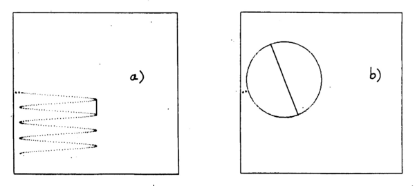
Figure 1 - Motion of a charged particle in the views parallel (a) and transverse (b) to B
The decay of the charged particle in event type 1 and 2 is a two body decay process, with the momentum of the charged decay product (q) being conserved by the unseen one (o). Use the knowledge of the momentum of the incident particle, and the conservation of momentum, to calculate the momentum of the “missing” i.e. unseen particle. Note that momentum is a vector quantity, and that only the initial injected particle is injected along the z direction.
Finally, use the law of conservation of energy to determine the mass of the charged decay product. The energy Ei of the incident particle is known from its mass and kinetic energy. It is equal to the sum of the energies of the charged (q) and uncharged (o) decay products. We also know that the mass M of any particle is related to its energy E and momentum P (cf.. the reminder window). One can solve the conservation law to obtain the mass of the charged particle (Mq) in terms of Mo , Po , Ei, and Pq. Show that
Thus, we do not have unique information at this point, but information on the pairs of masses, i.e., for a given value of the mass Mq there exists only one possibility of a mass for Mo.
Tabulate the value of the mass of the charged particle for various hypotheses of the mass of the uncharged particle, ranging from zero to the mass of the incoming particle. You can use Maple to help in your calculations. Repeat this for 3 events. You can look up this journal reference[3] or a list of known particles in a textbook to see which hypothesis agrees with your results. Note that if there is more than one neutral particle (which is the case for decays 4 and 5) then there will not be a definite mass for the neutrals, and we have to find alternate ways of determining the masses of the particles.
Part 2 - Determining Particle Lifetimes
Particles of a given type have identical properties such as mass, charge, etc. The quantum behaviour of elementary particles is manifested in their lifetime, i.e., the particles travel different distances before they decay. There is a statistical predictability associated with these decays, and following the rules of statistics we can determine a mean lifetime (or half life) associated with the decay. Read pages 30 ff. of the User's Guide to get a clear idea. Set the magnetic field to zero so that the charged particles traverse straight lines. Adjust the length of the chamber and the incident kinetic energy for maximal ease of measurement. Inject various particles and measure the path traversed before it decays (represented by a kink). Dividing the length by the velocity will yield the time it took before the particle decayed for that event. Repeat for 20 events for particle type 1 or 2. For particles that have not decayed within the chamber, add this time to the next event for a correct statistical treatment of the data. Plot the histogram of the individual particle lifetimes for a given type, and use the procedure outlined in the User's Guide to extract the mean (proper) lifetime. Remember to boost back from the lab frame to the rest frame of the decay particle using the factor of E/M (see e.g. Ref 2 for a refresher on boosting between frames). How does this agree with the values supplied?
References
- Onscreen Particle Physics User's Guide in the binder in the lab, and in OnScreen Particle Physics directory on the Desktop.
- Halliday, Resnick and Walker, Fundamentals of Physics; Wiley.
- F. Close, The Cosmic Onion, Heinemann Educational Books, 1984.
- J.W. Rohlf, Modern Physics from α to Z0; Wiley 1994.
- Physical Review D 50, Particles and Fields, Review of Particle Properties, p. 1173 ff. (1994).
- ↑ Onscreen Particle Physics User's Guide in the binder in the lab, and in OnScreen Particle Physics directory on the Desktop.
- ↑ Halliday, Resnick and Walker, Fundamentals of Physics; Wiley.
- ↑ Physical Review D 50, Particles and Fields, Review of Particle Properties, p. 1173 ff. (1994).
