Main Page/PHYS 3220/Rutherford I

Introduction

The Rutherford scattering experiment, where alpha particles (doubly charged Helium nuclei) were scattered off of a target (gold, aluminum, etc.) represents one of the most important experiments of this century. While the bulk of the alpha particles were scattered at small angles, indicating a soft collision process, a finite number of alpha particles however did scatter at very large angles. This could only have occurred though a collision with a massive object. From the distance of closest approach of the alpha with this object, and using information on the size of the whole atom, we came to know that the atom was mostly empty space. The results of this experiment formed the basis of subatomic structure, as we know it today – that the atom has a hard central core consisting of a tiny but massive core called the nucleus, surrounded by electrons, forming an electrically neutral system.

In this experiment we reproduce the results of Rutherfordby allowing alpha particles from a radioactive source (Am-241) to impinge on thin gold foil. We then compare the experimentally observed differential cross section (related to the number of detected alpha particles), as a function of the angle of scatter of the alpha particles off the target atoms. By comparing these particles to the theoretical expectations of elastic scattering of two particles, we can confirm that the alpha predominantly scatter off the nuclear core of the atom, and hence the structure of the atom is as Rutherford suggested.

Theory

Figure 1 - Particle scattering.

The theoretical analysis of the scattering cross section can be based on classical or quantum mechanics. In classical mechanics the number of particles scattered at a certain angle (θ) is a unique function of the impact parameter (b). We assume that a pure Coulomb potential is valid, but the appropriateness of this assumption shall be discussed later. To obtain the scattering cross section classically, first one solves Newton's equation of motion to obtain the relationship between impact parameter and scattering angle, and the results is that b α 1/θ. Small impact parameters thus lead to close encounters of the two charged objects, and thus large scattering angles. Conversely, distant collisions lead to small scattering angles. In quantum mechanics this relationship is not unique, but interestingly, a probability distribution arises for the particles to reach deflection angles θ that are synonymous with the classical answer (this is a special feature of the Coulomb potential). Although this relation tells us we are on the right track intuitively, unfortunately it is not very useful since we cannot measure b in any given interaction. We have to relate the scattered angle to something we can measure: the number of alpha particles scattered into the solid angle of the detecting device.

The number of particles scattered at a given angle depends on the change of the impact parameter with the scattering angle, and this can be verified from any book on modern or subatomic physics (e.g. ref 3,4). If the incident charged particle has charge Z₁ and energy E, and hits a target of charge Z₂, the Rutherford differential cross section can be written as

(1)

Q: Calculate the total cross section (hint: it diverges!!!). How is it that we continue to use this formalism when the prediction is infinity?

We have thus related the theoretical expectation (labelled Rutherford) to the measured variables. It is useful to review the article in Melissinos [1] as one can appreciate how careful experimental procedure is so crucial, and also the various factors that can affect the final result. There are several subtle (and some not so subtle) points one has to take into consideration for a meaningful comparison.

Apparatus

Read the Leybold manual first to make sure you understand the apparatus.

The apparatus consists of the scattering chamber, the vacuum system, the detector, and the data acquisition system. The components inside the scattering chamber necessary to perform the experiment are the source, two types of target foil (gold and aluminium) and two slits (1 mm and 5 mm wide). See the data sheets provided by Leybold for further details.

Figure 2 - Schematic of experiment.

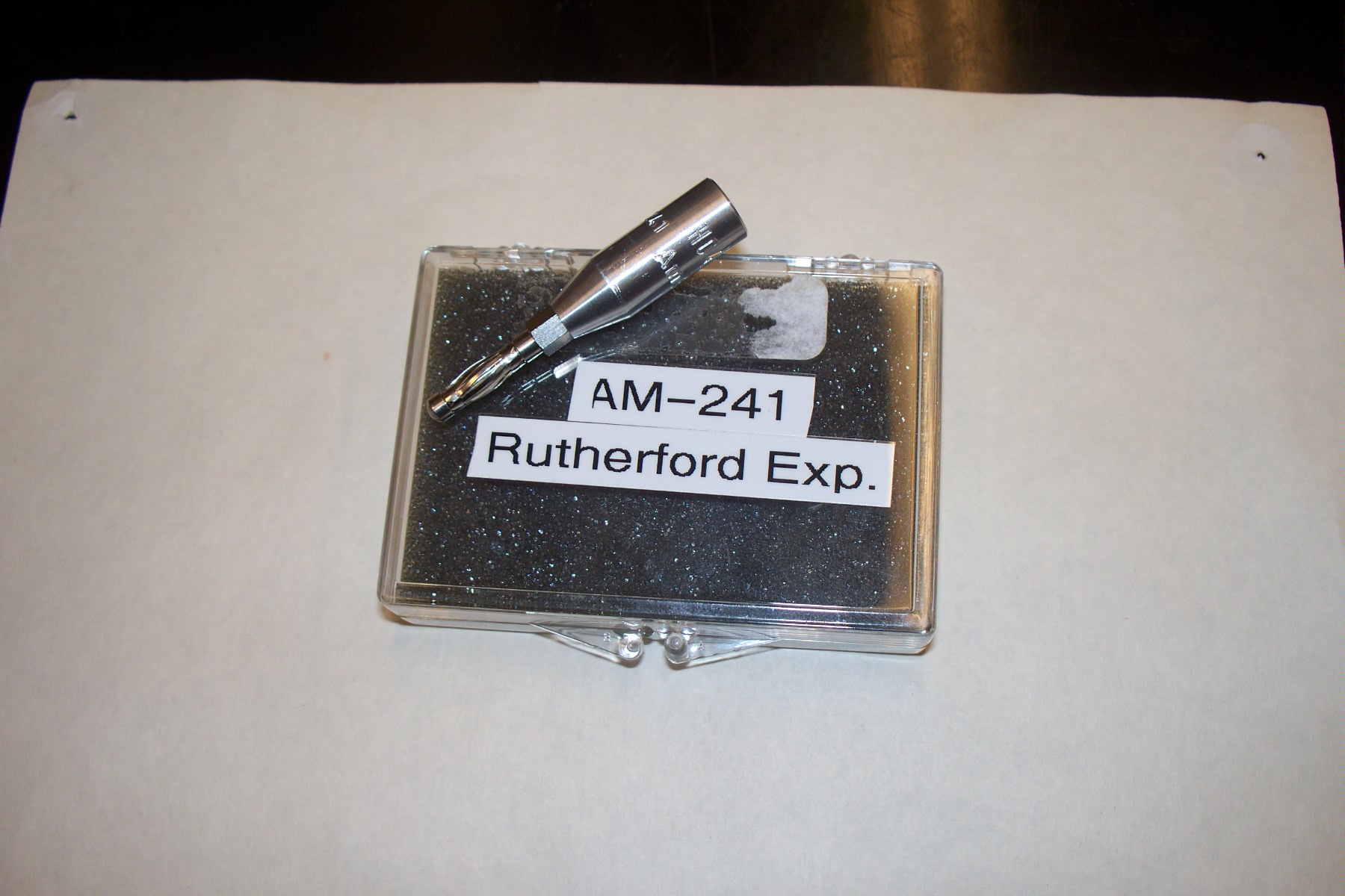
The source and slits

To install a foil please contact the TA or Lab Technologist.

Treat this source as you would any radioactive source: with care. Wear gloves when handling the source or when inserting the slits and target, and do not take it out of its protective container without supervision. The radiation from the source is emitted at all possible angles within the geometry of the container. To turn the radioactive source into a well-defined beam of particles one has to collimate the beam by using apertures. The source is placed in a metal holder so that the alpha particles emanate in a cone. A collimating slit is placed at a distance of about 2.8 cm from the front face of the metal holder, and a metal foil of a few microns thickness is placed in a holder in front of the slit, directly against it (the drawing is exaggerated), i.e. further away from the source than the slit. Here “front” is defined by the direction of the alpha particles if they were unimpeded in their direction of travel from the source through the collimator. The detector is 2.7 cm in front of the foil. The source-foil assembly can be rotated about an axis that passes through the foil, while the detector is fixed. This is equivalent to a fixed source-target assembly and rotating the detector. The central axis of the detector should point along this axis of the foil-source assembly at zero degrees. In practice, any errors of this may cause an overall shift in the result, as we shall discuss later.

The detector

The detector is a silicon (solid-state) device, and has a slit on its face of height ( height 7mm x width 1.5mm. The detector is connected to a pre-amplifier (to amplify the weak signal) and discriminator, and these are set to generate definite pulses when a pulse generated in the detector exceeds a certain threshold (as defined by the discriminator). A A digital counter records the shaped pulses. This way one can suppress unwanted background sources (although light hitting the detector could also trigger events). If one sets the threshold too high, one suppresses of course some events of interest, but this should at worst lead to a reduced count rate, but not necessarily affect the outcome of the experiment. Can the dis. threshold be adjusted?

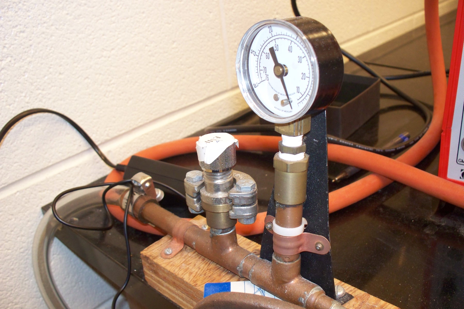
The vacuum system

There are several sets of measurements using the chamber. In between each stage, the chamber must be returned to normal atmospheric pressure so that the lid may be removed. Hence the process of evacuating the chamber, and returning it to normal pressure, are described at first. Practice with no foil in the chamber and test that the lid of the chamber is secure when the chamber is evacuated.

Figure 3 - Vacuum system Schematic.

Figure 4 - Vacuum system.

Evacuating the scattering chamber

Please be gentle with the valves at all times the foil is delicate and very expensive to replace. Never touch the foil directly as it is easily perforated, and take it or out of the holder very gently. Carry out the vacuum operation slowly. Always replace the foil in its container bag in between steps.

1. Open B check for secure lid slowly (if it is not open). Close A.
2. Turn on the roughing pump until the vacuum reaches 70 mm of Mercury.
3. Slowly close B.
4. Turn off the pump.
5. NOTE this is very important! Open A (this is to avoid back pressure from the pump and oil from entering into the system).

Releasing the chamber to atmospheric pressure

If the foil is in the chamber, make sure that the foil is perpendicular to the chamber valve when returning the vacuum to the normal pressure or evacuating the chamber.

1. Close A. Open B slowly.
2. Open A slowly.

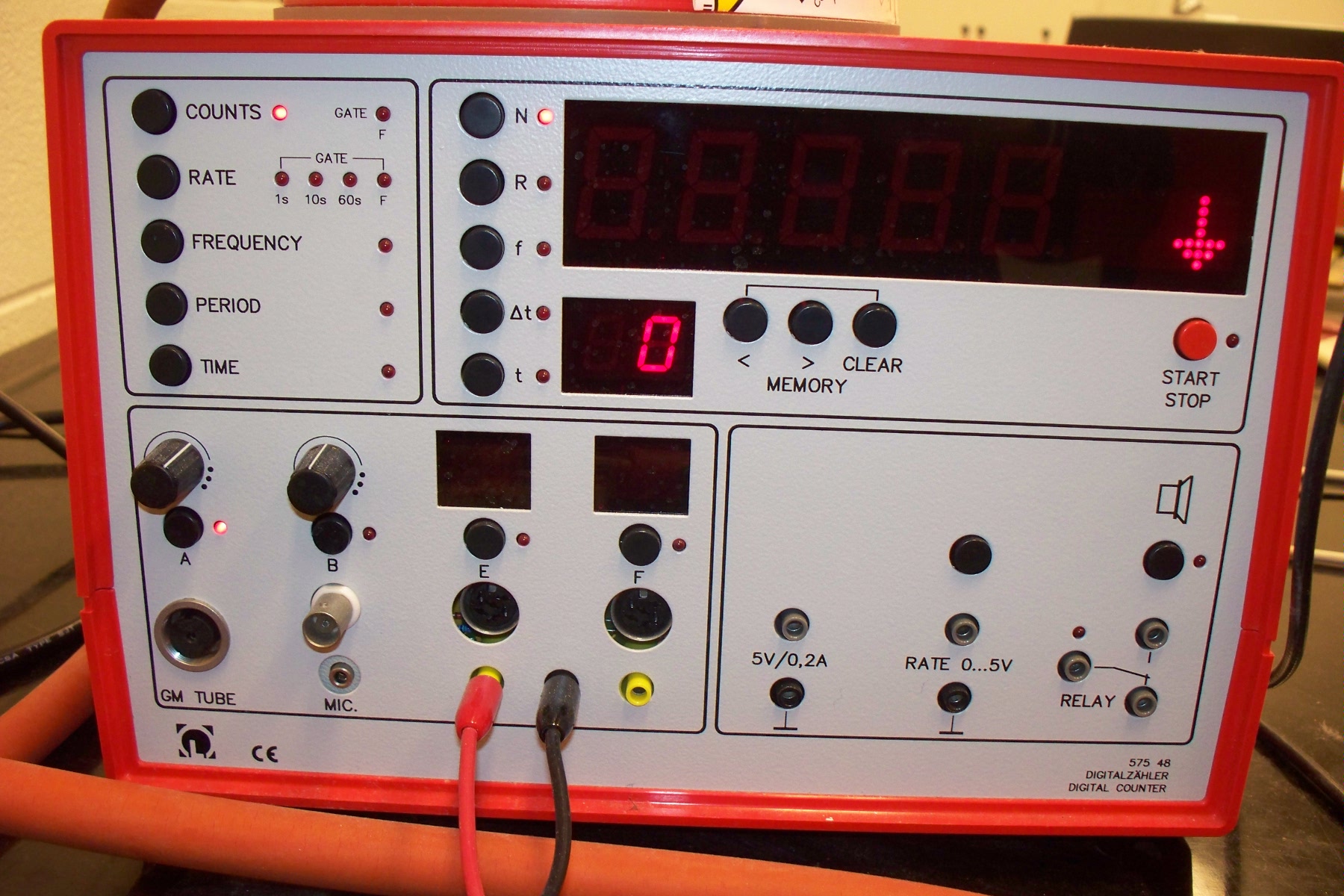
Data Acquisition System

Note: There are two ways of recording the data: “rate” and “counts”.

A computer interfaced data acquisition system is provided, which can display on-line the Poisson statistical analysis of the recorded events. One might think that measuring the count rate 10 times (for a given time interval), and deducing the average and deviation would be sufficient. However, due to the statistical nature of the radioactive decay process we do not have a constant beam of particles; also the scattering itself is a probabilistic process. Such random events are obeying Poisson statistics. The computerized data acquisition system allows one to collect data in 10-second or 60-second intervals and to assemble a histogram (to be compared with a Poisson fit) and to display graphically the collected count rate. A function is provided to deduce the average count rate and deviation from the data.

Required Components

1. Protractor
2. Control Box
3. Counter
4. Radioactive Detector
5. Vacuum Gauge
6. Slits
7. Source
8. Vacuum Pump

Here are some definitions that may prove to be useful:

The number of scattering centres in the target is related to the thickness of the foil and the density of the material via N0 = (a x d) x ρ x A₀/ A , where

• A₀ = Avogadro’s number = 6.0222 x 10²³ atoms /mole.
• A = atomic weight of the target in g/mole.
• ρ = density of the material (19.3 g/cm³ for Au, 2.7 g/cm³ for Al).
• d = thickness of the target (2 micrometers = 2 microns for Au, 7 microns for Al).
• a = area of the target intercepted by the beam.

(N is the same as in Melissinos but note our N0 is not the same as Melissinos N0, which is the Avogadro’s number(A₀ here)).

The activity of the AM-241 alpha source is 330 kBq.

Procedure

We stress again that you must understand how the vacuum pump operates. Misuse can lead to destruction of the whole apparatus (oil flooding, tearing of the foils etc. ).

1. Using a 5mm slit and no foil, find the “zero angle” (θ₀ ) of the apparatus by recording the counting rate of the alpha particles for several angles (-10^o to +10^o), starting from the zero on the dial angle indicator (chamber lid). Take measurements for negative and positive angles in increments of 2.5^o (half of the smallest division on the dial).
2. Place the Gold foil together with the 5mm slit on the mount and acquire measurements of counts for the following angles 10, 20, 30, 40, 50, 60 degrees with respect to θ₀. Make sure you obtain at least 10 counts for each of these angles.
3. Repeat the above using the Aluminium foil with the 5mm slit.
4. Use the 5mm slit to take background measurements (do not place any of the foils) for the same angles as in step 3 and use this date to correct for the above measurements. The small angles (<30^o) should not take too long. However, as you reach the large angles, the time necessary to obtain enough readings can be substantial. Make sure you take at least 1 count for each of the angles (for the small angles you can probably take a few hundreds in a matter of seconds).

Plot the log(rate) vs. log(sin⁴θ/2) with appropriate conversion to radians. Derive the relationship between the observed rate and the cross section. What do you expect for the behaviour of this graph? Using the relationship between the rate and the Rutherford cross section formula (equation1), find the ratio of atomic numbers between Gold and Aluminium.

References

1. Melissinos, Experiments in Modern Physics, Academic Press.
2. Preston and Deitz, The Art of Experimental Physics, Wiley and Sons.
3. H. Frauenfelder and E. Henley, Subatomic Physics, Prentice Hall.
4. A. Das and T. Ferbel, Introduction to Nuclear and Particle Physics, J. Wiley.