Difference between revisions of "Main Page/PHYS 4210/Fourier Optics"
| Line 57: | Line 57: | ||
<table width=500 align=center><td> | <table width=500 align=center><td> | ||
| − | <p align=justify>[[File: | + | <p align=justify>[[File:FO_Fig1av2.PNG|500px|border|center]] |
<b>Figure 1a </b> | <b>Figure 1a </b> | ||
<br clear=right> | <br clear=right> | ||
| Line 63: | Line 63: | ||
</td></table> | </td></table> | ||
<table width=500 align=center><td> | <table width=500 align=center><td> | ||
| − | <p align=justify>[[File: | + | <p align=justify>[[File:FO_Fig1bv2.PNG|500px|border|center]] |
<b>Figure 1b -</b> A lens provides a Fourier Transform of the image in its focal plane. | <b>Figure 1b -</b> A lens provides a Fourier Transform of the image in its focal plane. | ||
<br clear=right> | <br clear=right> | ||
Latest revision as of 14:38, 19 January 2015
Fourier Optics
In this experiment we investigate the diffractive (as opposed to refractive) properties of a lens, named Fraunhofer diffraction. A HeNe laser is used to illuminate an image or a grating whose Fourier image is generated in the focal plane of a lens. The Fourier image is modified by cutting away low or high components (orders of the diffraction pattern) and a second lens is used to view the altered image.
Key Concepts
|
|
Introduction
Ray optics deals with the simple design of optical systems. While trying to take, e.g., a microscope to its limit, i.e., to improve the resolution, researchers in the middle of the 19th century (Abbé, in particular) found that the dark parts of the image inside an optical system contribute to the final image. Physical optics makes use of the wave nature of light to understand these phenomena. It turns out that a simple lens produces in its focal plane a diffraction pattern for the image. In ref. 1 detailed explanations of the mathematical description of imaging are provided.
The problem is summarized in Fig. 1, which shows how parallel light illuminates an object, and a symmetric set-up of two high-quality lenses. The first lens is used to construct a Fourier image in the focal plane, while the second lens forms back the image. The diffraction pattern in the focal plane (the drawing is rather artistic, i.e., inaccurate) is easily observed for monochromatic light (a mercury lamp with a colour filter, or a laser), and can be modified (filtered) to modify the image.
The description of the pattern in the focal plane becomes straightforward if we consider a simple image, such as, e.g., a grating. From previous optics demonstrations you may be familiar with two types of gratings that are characterized by their line density (in lines/inch): (i) simple rulings (e.g., Ronchi rulings for the measurement of the resolution of lenses and their spherical aberration) have an intensity profile that corresponds to a square-wave pattern; these rulings when illuminated by a monochromatic source generate a diffraction pattern of many equidistant dots along a line perpendicular to the rulings; (ii) gratings with a sinusoidal intensity patterns are often used to produce a single pair of diffraction maxima. This corresponds to the Fourier representations of a sinusoidal intensity pattern: a single cosine mode (central spot) and two sine-terms, while the Fourier series for case (i) has infinitely many contributions.
The location of the diffraction maxima depends on the spacing of the ruling d and the wavelength λ of the light. A useful parameter that appears in the intensity patterns of apertures is given by
|
| (1) |
- The amplitude of the diffracted light is given by a Fourier transform of the aperture function F(y) which equals to one for perfect transmission and vanishes for a perfect blockage of light (ref. 4, p 131):
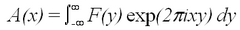
(2) - For some aperture functions the calculation of the diffracted light intensity is straightforward. A Maple worksheet is provided with examples of a diffraction grating (cosine-squared modulated transmission grating function F(y) and step-function pattern F(y) for a line ruling usually referred to as a Ronchi ruling).
- The mathematical description of the transform of a sinusoidal or square-wave intensity pattern is straightforward and is done in standard courses on advanced calculus (see ref. 3). The pattern for a cosine-squared aperture function F(y) = cos2(πy/d) consists of a central peak and two side peaks located at
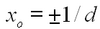
(3)
The side peaks have an intensity of about a quarter of that for the central peak. For a square-wave aperture function (Ronchi ruling) peaks of nearly equal intensity occur at x = 0 and at x0 = ±1/d followed by peaks of decreasing intensity for x1 = ±3/d , x2 = ±5/d , etc. Weaker peaks arise at interspersed locations if the square-wave aperture is not symmetrical, i.e., if the rulings are of slightly different thickness than the gaps.
The amazing observation from figs. 1 a, & b is that a simple optical set-up provides instantaneous Fourier transforms. It is, therefore, referred to as a coherent optical computer.
 Figure 1a
|
 Figure 1b - A lens provides a Fourier Transform of the image in its focal plane.
|
One application of the Fourier image technique can be found in filtering of images for printing (e.g., the removal of graininess). The resolution of printers is typically in the range of 300-1200 dpi (dots per inch) for conventional laser printers and reaches 24000 dpi in professional typesetters. In the second part of the experiment we demonstrate the effect of removing high Fourier components of an image.
Some of the questions that should be understood are raised and answered in refs. 1 and 4:
Comparison of strictly periodic vs. non-periodic images.
The Fourier series representation that is valid for a grating (that is assumed to be composed of infinitely many lines, i.e., truly periodic) goes over into the Fourier transform, i.e., the spatial signal is not composed of discrete multiples of a basic frequency, but a continuous spectrum of spatial frequencies is present.
Why do we observe a Fourier pattern in the focal plane?
It is mathematically evident that a periodic square-wave signal (in our case in the spatial domain) can be decomposed into sine-contributions with multiples of a discrete frequency. Why does the image in the focal plane contain dots that correspond to the Fourier contributions (location and intensity are determined by the frequency and amplitude of the Fourier representation)? This is demonstrated in the chapter on diffraction theory: a Fraunhofer diffraction pattern of an aperture (or obstacle) is equivalent to the Fourier transform of the function describing the aperture. Ref. 4 uses a physically intuitive approach with phasor diagrams.
What does one obtain for two-dimensional images?
The previous discussion of rulings and gratings was simple in that they represent one-dimensional objects, i.e., there is no information content in the dimension along which the lines, in principle, are infinitely long. In general, however, an image does contain two-dimensional information. In the simplest case we cross two gratings and observe that the diffraction pattern becomes two-dimensional, namely a product of the two orthogonal patterns. Thus, for arbitrary images the lens produces a two-dimensional Fourier transform (Fourier series for periodic images).
What is the effect of high-pass or low-pass filtering of images?
One can consider for any image the question of information content at high and at low spatial frequencies. For half-tone printing (production of greyscales by printing black dots with varying density) one makes use of the limited resolution of our eyes: without magnification the eye perceives only the low-frequency components that carry the interesting information of, e.g., a photograph. Magnification of the image makes, however, the dots visible. It is possible to mask the image in the Fourier transform plane with a low-pass filter, i.e., to remove the high-frequency content to produce a soft image. Conversely, high-pass filtering and artificial modification (introduction of detail by blocking every second Fourier component, see ref. 2) is easily accomplished.
Experimental Procedure
WARNING: Laser light can easily damage your eyes! Never look directly into the beam or at bright images of the spot that are produced on metallic or mirror surfaces! Wear protective glasses when operating the laser. While operating the laser a sign should be posted on the door to warn people entering the room about the presence of laser radiation.
First you should gain familiarity with gratings, rulings and the basic set-up. Two separate HeNe lasers are used in this experiment. The first one is used to direct its beam at gratings and Ronchi rulings with a screen for a manual recording of the pattern as well as detection of the intensity of dots using a photodetector/amplifier/voltmeter set-up. The second laser in our experiment is focussed onto a 10μm pinhole with adjustable micrometer screws. Three identical lenses are provided in order to realize the 4f-focussing set-up of Fig. 1. They are, in fact, good-quality two-element lenses with chromatic correction, a resolution of 32 lines/mm and have all a focal length of 350 mm (cf.. the Optikon specification sheet). The first lens acts as a condenser to provide a parallel uniformly illuminated beam. Adjustments of the three micrometer screws may be required to obtain a proper illumination of the image slide. Be careful, however, not to ‘lose’ the laser spot altogether. The second lens produces a Fourier image in the focal plane (where low-pass filtering can be applied using an aperture). The third lens is used to convert the (modified) Fourier image again into a normal (filtered) image.
- Observe the function of high-density gratings (square-wave and sinusoidal intensity patterns with thousands of lines per inch) as they are mounted in a laser beam (use the laser without a pinhole). Take measurements for slides A and B and determine their type and line density. Repeat the measurement using Ronchi rulings with hundreds of lines per inch. The wavelength of a HeNe laser equals 632.8 nm. A diode laser (e.g., in a laser pointer) has a wavelength of 675±10 nm. Record the spacings as produced on a screen at a fixed distance, calculate diffraction angles θn, and calculate d for the given grating. Comment on the observed pattern. A MATHEMATICA worksheet is provided in the Appendix for the calculation of diffraction patterns with a finite number of slits.
- Observe the laser set-up with a pinhole. Place Ronchi rulings with tens of lines per inch or simple slides with rulings between the condenser lens and the first imaging lens. Place a screen into the focal plane and observe the diffraction patterns. Estimate the separation of the spots and compare your results with eqs. (1,3). Are there infinitely many Fourier components?
- Place a grid-shaped ruling between the condenser and imaging lens. Observe the Fourier image as well as the regenerated image on the screen. Place slits of different widths in the focal plane to cut out high Fourier components first in the horizontal, then in the vertical planes. It is possible to completely remove one set of lines. Rotate the slit in the Fourier plane by 45 degrees. What do you observe? Explain this in your write-up.
- Place a low resolution image slide into the holder and observe the results. Apply a low-pass filter to remove the graininess. Record images with and without filtering using a camera and provide explanations including some mathematical detail (Fourier-series analysis for periodic images in one dimension is sufficient but Fourier transform analysis can be done easily with Maple or Mathematica).
Using laser set-up 1 (no pinhole):
Using laser set-up 2 (with pinhole):
References
- E. Hecht, Zajac, Optics, Addison-Wesley.
- Gillespie, Optical Information Processing, Phys. Educ. 29, 127-34 (1994).
- G.A. Arfken, Mathematical Methods for Physicists, Academic Press.
- F.G. Smith, J.H. Thomson,Optics, 2nd ed.
Appendix
MultipleSlitDiffractionPattern.nb (copy and paste into a Mathematica Notoebook)
Manipulate[
Plot[{((1/n) ChebyshevU[n - 1, Cos[b k/2]] Sinc[a k/2])^2,
Sinc[a k/2]^2}, {k, -kmax, kmax},
PlotRange -> {0, 1},
Axes -> False,
Frame -> True,
FrameTicks -> {True, False},
FrameLabel -> {"position", "intensity"},
PlotLabel -> ToString[n] <> " slit diffraction pattern",
Filling -> {1 -> Axis},
PlotStyle -> {Automatic, {Thick, Dashed}},
ImageSize -> {500, 350},
ImagePadding -> {{40, 20}, {40, 20}}],
{{a, 0.5, "slit width"}, 0, 1, Appearance -> "Labeled"},
{{b, 2.5, "slit spacing"}, 1, 5, Appearance -> "Labeled"},
{{n, 2, "number of slits"}, Range[10], SetterBar},
Delimiter,
{{kmax, 10, "horizontal range"}, 1, 100, Appearance -> "Labeled"}]