Main Page/PHYS 4210/Gamma Ray Spectroscopy
Gamma Ray Spectroscopy
In this experiment we study the gamma ray spectra of several radioactive elements to learn about the interaction properties of gamma rays with matter. The gamma rays are detected through ionization of the material in a scintillation counter, and the output pulse, which is generated with a photomultiplier tube, is then recorded with the aid of a Multi Channel Analyser (MCA) connected to a computer interface. The different types of interaction of gamma rays with matter are understood from a detailed analysis of the observed spectra. Thus, this experiment not only illustrates the physics of the interaction properties of photons, but also introduces scintillation detectors and relevant electronics.
Key Concepts
|
|
Introduction
Gamma rays are photons of very short wavelength (~10-12 cm) or very high frequency (1022 Hz) that are emitted during nuclear transitions. The decay schemes of the three radionuclides that we study (Na22, Cs137, Co60) are shown below. Read ref. 1-5 to get a clear idea of the significance of the gamma energies.
 Figure 1 - Decay schemes of Cs-137, Co-60, and Na-22.
|
Method
Photons are electrically neutral, and unlike charged particles, do not experience the Coulomb force. They are, however, carriers of the electromagnetic force, and are able to ionize atoms through their interaction with matter, and this leads to the deposition of energy in the medium as the ionized particle slows down in traversing the medium. This energy can then be detected. The three modes of interaction are: photoelectric effect, Compton scattering, and pair production where the photon interacts with an atom, an electron, and a nucleus respectively. You should read the details of each type of interaction in the references and include this in your write-up. We summarise it briefly below.
Photoelectric effect
The photon of energy Eg is absorbed by an atom and an electron from one of the shells is emitted. If Be is the binding energy of the electron, then the energy of the emitted electron will have an energy Ee = Eg - Be. Since Be is small (of the order 40 KeV) compared to Eg (of the order 1MeV), the electron carries most of the energy of the photon.
Compton scattering
The photon scatters off an electron that is either free or is loosely bound in the atom, thereby scattering the electron. It can be shown (do so in your writeup) that the energy of the scattered electron is related to that of the incident photon, the angle of the scattered photon (theta), and the mass of the electron me through the relationship:
 | (1) |
 Figure 2 - Compton scattering.
|
Hence the scattered photon (of energy hv’) has the freedom to move at any angle with respect to the incident photon (or gamma ray, as we call it here), whereas the scattered electron is bound by the laws of conservation of momentum to only go in the forward direction. The kinetic energy of the Compton electron is EC = hv- hv’. This, combined with the above formula for the energy of the electron shows that the maximum kinetic energy of the electron is when theta = 180° ,i.e., when the photon is scattered backwards. This maximum is known as the Compton edge.
Pair production
If the photon has more than twice the rest mass of an electron (0.511 MeV), the photon can produce an electron-positron pair. This must be done in the Coulomb field of the nucleus to balance linear momentum, as the photon cannot produce a pair in free space (its center of mass would have zero momentum). The energy in excess of the rest masses of the products is imparted as kinetic energy.
The energy dependencies of the three processes are quite different. At energies below a few KeV, the photoelectric effect dominates and the Coulomb effect is small, while pair production is energetically impossible. For the region of 0.1 to about 10 MeV, Compton scattering dominates. Above this, pair production is the predominant method for the interaction of the photons. It is important to realize that in photoelectric effect and pair production, the photon is eliminated in the process of the interaction, whereas in Compton scattering, the energy of the photon is only degraded. As explained further below the various processes involved lead to a complete or incomplete energy deposition of the gamma energy in the scintillator. We have to be concerned only with the first two methods; the photoelectric effect leads to complete energy deposition, while the Compton effect can lead to processes where the scattered gamma ray leaves the detector without depositing its energy.
The Radioactive Sources
You will be working with five radioactive sources: Mn-54, Na-22, Cs-137, and Co-60. You should note the radiation dosage and date marked on the source, and read about radiation safety and how to handle radiation sources from ref. 1, pg 326-328. Calculate the number of disintegrations per second for each of the sources based on the quoted dosage.
The Detector
The gamma rays that are emitted from the source are detected with a scintillator detector. In our laboratory, we use inorganic crystals of sodium iodide doped with impurity centres of thallium. This combination is denoted by NaI(Tl). A photon entering the detector ionizes the material through the processes described above. The positive ions and electrons created by the incoming photon diffuse through the lattice and are captured by the impurity centres i.e. the Tl atoms, which act as luminescence centres. Recombination produces an excited centre,which emits visible light upon its return to the ground state. The efficiency of these inorganic crystals is high, but the light output is spread over a time interval of the order of microseconds.
In general, for gamma rays less than 1 MeV, photons undergoing the photoelectric process will be completely absorbed and will give rise to a determined number of light quanta. These light quanta are then seen by the photomultiplier tube, and the output pulse will be proportional to the incoming energy of the gamma ray. The energy of the electrons produced by the Compton effect will depend on the angle at which they are scattered and hence there will be a spectrum of detected pulses. At energies above 1 MeV, pair production can occur and the electron and positron lose their kinetic energy by ionizing the medium. The electron is absorbed, while the positron annihilates within a few nanoseconds into two photons, each of 0.511 MeV. These may then interact through the photoelectric or Compton effect. There are three possibilities for the observed energy (show this in the writeup) depending on whether none, one or both of these photons from the positron annihilation are detected.
As mentioned, the produced light is proportional to the energy of the incident gamma ray. This light is then made incident on the photocathode face of a photomultiplier tube (PMT), which converts the photons to photoelectrons through the photoelectric effect. The electrons are amplified and then converted to a voltage pulse. The PMT used here has 10 stages and the multiplication for such tubes is about 106 for an operational voltage between the cathode and the anode of 1000V. The cascade of electrons produced at each of the multiplication stages of the dynodes is collected at the anode, converted to a voltage pulse, which is then amplified and analysed. The PMT is enclosed in a high permeability material to shield against magnetic fields, as such effects would affect the efficiency of the tube.
Note that the metal shield that encloses the scintillator crystal does not allow β (or other charged) particles to permeate and deposit their usually well-defined energies. Thus, you should not expect to observe structures associated with, e.g., the 0.514 MeV and 1.17 MeV electrons coming from the Cs137 source with branching ratios of 93.5% and 6.5% respectively (cf.. Fig. 1). Charged particles are created inside the crystal by γ ray impact. There will be, however, backscattered γ rays from Compton scattering outside the crystal, e.g., off the backing of the source and off the lead shield.
Read the specifications for the model of the scintillator detector and photomultiplier that you have. Note that the size of the crystal is small. How does this affect your results? The typical quantum efficiency of scintillators of this type is one photon of light produced per 100 eV of energy deposited in the scintillator. The width of the full-energy peak (i.e. when the gamma energy is fully absorbed) depends on the number of light quanta produced by the incident gamma ray. The energy resolution, dE/E is an important quantity to consider as this factor will determine if we can separate gamma rays very close in energy.
The chain of events may help illustrate this point. The incident gamma ray of energy Eg produces a photoelectron with energy Ee ~ Eg. The photoelectron produces N light quanta in the scintillator material via ionization and excitation, each with an energy Elq. Since the light is visible (~400 nm), Elq is about 3 eV. This light falls on the photocathode, which has a quantum efficiency or sensitivity to the wavelength of the incident light. For the tube supplied, the efficiency peaks near 400 nm, making it quite suitable for use with a scintillator. Let
- ε(light) be the efficiency for the conversion of the excitation energy into light quanta
- ε(coll) be the efficiency for collecting the n lq light quanta at the photocathode of the PMT
- ε(cathode) be the efficiency for the cathode to eject a photoelectron
Then, the number of photoelectrons produced at the photocathode is
 |
Typical values for the efficiencies for NaI detectors are:
- ε(light) = 0.1
- ε(coll) = 0.4
- ε(cathode) = 0.2
For a 1MeV gamma ray, this yields about 3x10³ photoelectrons at the photocathode. All the processes mentioned above are subject to statistical fluctuations, and contribute to the broadening of the line width. In addition, there is a contribution from the statistical process due to the multiplication of the photoelectrons in the stages of the PMT.
The Multichannel Analyser (MCA)
The electrons collected at the anode of the PMT pass directly into the Spectrum Techniques MCA (UCS 30). This pulse of electrons enters the internal pre-amplifier, followed by the internal amplifier. The voltage across the internal amplifier resistance is digitized into one of 1024 bins according to its maximum value (peak height)- this process of converting an analog voltage into a digital value is called analog-to-digital conversion (ADC). The MCA performs this task for all pulses and creates a histogram of counts in each ADC bin.
There are several important parameters which affect the performance of the MCA. For a detailed explanation of the pulse processing details refer to the book by Knoll, "Radiation Detection and Measurements" listed in the references section below.
- Amplifier Gain: This is an amplification factor applied to the detector pulse using the adjustable coarse gain and fine gain controls.
- Lower Level Discriminator (LLD) : The amount above the average background which is required for the MCA to accept a particular pulse and record its statistics in the histogram.
- Run Time: The actual length of time for which to acquire data.
- Live Time: The time the detector is actually able to detect pulses.
- Dead Time: The time during collection when the detector is unable to process additional events. Look up live time and dead time and discuss in your report.
- High Voltage: The parameter "high voltage" in the MCA client software does nothing. Bridgeport makes an HV supply for PMTs which connect directly to the eMorpho. We are using a separate power supply, hence adjusting this parameter in the software does nothing. However, changing the 1000V supplied to the PMT from the power supply will mean that more electrons are collected per pulse. If this dc voltage is set too high and and too many photons are present, there could be a buildup of charge inside the PMT and catastrophic damage could occur.Please do not change the setting of the voltage to the PMT from 1000V.
Turn the power on the spectrum analyzer (UCS 30) and run the program "USX" located on the desktop. (The UCS 30 manual is located on the desktop and should be referred to for additional information.) Hover over the toolbar icons and note the descriptions. Click on each icon and note the options available. For example, you can toggle between a linear and logarithmic y-axis scale by clicking on the "y-log" icon on the toolbar. Additionally, during data collection you can adjust the scale of the y-axis by scrolling up and down when the mouse is in the graph region. Review the operation section (pg 16-25) of the UCS30 lab manual.
The signal from the PMT is directly input to a multichannel analyser which is a device that sorts incoming pulses according to pulse height and keeps count of the number at each height in a multichannel memory. The contents of each channel is displayed on a screen to give a pulse height spectrum, which is then analysed. The amplitude of the incoming pulse is digitized with an Analogue to Digital Converter (ADC), and sorting is done based on how many pulses had a particular value of the digitized amplitude. The total number of channels into which the voltage range is digitized determines the resolution of the MCA. Refer ref. 1, 2 and 4 to understand the characteristics of the electronics you are supplied with, and to learn more about the ADC range and resolution that can be achieved. Also, use ref. 1, 2, 4 to understand the functions of a MCA. Review what is meant by ‘dead time’ and ‘live time’. Do not operate with a dead time of more than 30%, since too high count rates can cause the electronics to misbehave.
The natural linewidth of the gamma rays is extremely narrow (a few eV compared to the MeV range of the energies themselves!). The broadening observed in the recorded spectra is a result of the detection method (a cooled Germanium detector would show these lines being much narrower, but again at a resolution that depends on the detector itself). It is important to realize on the example of the Cs137 spectrum, for which a single energy at 0.662 MeV is expected that several effects occur in ‘real life’:
- Broadening of the photopeak at 0.662 MeV.
- A Compton background (plateau) with two edges: at the higher end, below the
photopeak a maximum electron(!) energy of
Understand this result using eq. (1). At lower energies in the Compton plateau a distinct photopeak corresponding to backscattered gamma rays whose energy follows from eq. (1) for θ = π. Note how nearly backscattered gammas give about the same energy due to the slow variation of the cos function for θ = π.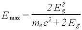
(2) - A fluorescent K-shell Xray peak caused by soft gamma rays hitting the shielding material (typically lead), knocking out K-shell electrons. The vacancies are typically filled from the L-III shell (2p±1). Use the CRC Handbook (see Lab Technologist or Library) to verify that the difference in energy results in characteristic X rays of about 75 keV for Pb.

A typical spectrum is shown in Fig. 2 on a linear scale. If we go to a logarithmic scale (the MCA software allows to do this), we find an additional weak peak at about twice the gamma energy. This is the so-called sum peak, which arises when two gamma rays from uncorrelated decay events are depositing their energy in the scintillator within a fraction of a microsecond, i.e., the timescale over which the scintillation in the crystal and photomultiplication in the tube occurs. You should be able to observe sum peaks in this experiment when accumulating enough statistics. The peaks appear more strongly when the source is brought closer to the PMT.
 Figure 3 - Typical Cs-137 spectrum using an NaI(T1) scintillator.
|
Besides sum peaks another complication can occur for high-energy gamma rays. When pair creation is an important energy deposition mechanism, so-called escape peaks are observed. These correspond to events where one or more of the created electrons/positrons escape the crystal without giving up their energy. Such peaks occur at Eg - j (0.511 MeV), where j is the number of escaped electrons/positrons. Since we do not use sources with Eg > 2 MeV in this experiment, we do not find this complication in our spectra.
Experimental Procedure
While conducting the experiment, make sure that only the source whose spectrum you are observing is near the apparatus otherwise your calibration results will be skewed. Take only one source out at a time, and keep the others in the box away from the detector. Be careful while handling sources. Become familiar with the documentation and all the apparatus before starting.
Ensure the following connections: the scintillator and PMT are connected, the HV output from the PMT is connected to the USC 30, the signal output from the PMT is connected to the MCA, and the MCA is connected to the computer.
In our setup, we have mounted the PMT vertically, allowing you to place the source on a tray at several different distances from the source. Once you have found an optimal distance for all three sources (i.e. you do not get ‘pile up’ effects (see Leo)), it is best to use this distance for calibration and determination of the peak energies. However, in the last part of the experiment you will be asked to draw qualitative conclusions by placing a source at varying distances.
Settings
Please ensure the following running parameters
- High-Voltage to PMT: +1000V (Click on the "Amp/HV/ADC" icon on the toolbar to set and turn on the voltage.)
- Amplifier Gain: Use the course gain and fine gain controls to set the gain in the range of 16 - 18.
- Conversion Gain: 1024
- Peak Time: 1 micro sec
 Figure 4 - Gamma source, NaI(T1) detector, PMT, lead shield showing relevant processes.
|
Use Experiment 2.1 as a guide for gamma ray calibration from Duggan in the red binder in the lab. The UCS 30 software will only be used for data collection and observing the spectra. All data analysis, including energy calibration, can be conducted using software like Excel or Mathematica. Use the 4 known sources Cs-137 (0.662 MeV), Co-60 (1.173 MeV, 1.332 MeV), Mn-54 (0.835 MeV) and Na-22 (0.511 MeV) provided in the RSS 8 radiation source kit (Spectrum Techniques). Centre each source (label down) about 5 cm from the face of the detector and collect a spectrum for at least 5 minutes with each source. Longer collection times correspond to smaller statistical errors, why? Stop collection prior to saving and record the dead time, live time and real time for each spectrum. Save the spectrum. (The .csv file generated contains a single column with the UCS 30 parameters in the first 18 rows followed by the spectrum data (number of events) in each channel from 0 to 1023. Create a calibration curve using all five sources i.e. for each spectrum locate the channel number corresponding to the gamma ray energy peaks and create a plot of the energy of each peak and the peak channel number. What is the error of a straight line fit to this curve? If the fit is poor, you have made a mistake in assigning peak-channel values, and may have to repeat the analysis. Discuss sources of error.
Using your calibration fit plot the calibrated Cs-137 spectrum, Co-60 spectrum and Na-22 spectrum separately(i.e. events as a function of energy). Explain all the peaks on the spectra. Do you see any 'sum peaks’? (Plot your data on a logarithmic scale for a better view!) Explain why this peak occurs. Does it occur at the value you expect? What is the source of the 511 keV peak in the Na-22 spectrum? The Na-22 has a gamma ray energy at 1275 keV. What value of the maximum position do you find based on your calibration curve? Is this consistent with the resolution dE/E? What is the present activity of these three sources (note the date marked on the source)? Present the calibrated spectra in your report and explain all the interesting details.
Put a sheet of lead on the shelf and then place the Co-60 source above. How does the spectrum change? Now place the sheet of lead on top of the source. What, if anything, has changed in the spectrum? You may have to move the source closer or farther from the detector to observe the backscattering signals. Collect a spectrum for each case for a sufficient collection time and save. Caution: Always wear gloves when handling the lead sheets.
- Obtain the energy resolution for the photopeak for Cs-137 and for one of the Co-60 peaks (See Knoll, chapter 4). Does this agree with what you have learned about scintillator devices?
- Place the Cs-137 source at varying distances from the detector and explain qualitatively the rates that you observe. Put the source at slot 2 below the detector, and place first one, then two, and then three sheets of lead on top of the source. Comment on the rates, and the reason for the observed behaviour. Repeat for sheets of aluminum.
- A spectrum of the unknown source (the background in the room) will be collected by the Lab Technologist. The data will be saved and the file can be found in the "data" folder located on the desktop. Using this data, create a calibrated spectrum using your calibration fit. Use your now-calibrated gamma-ray spectrum to identify the radioisotope(s) found in the background.
- After all data has been collected, turn the HV off from the software controls and then turn off the UCS 30 power switch.
Calibration Curve
Gamma-ray Experiments
References
- Preston and Dietz,The Art of Experimental Physics, Wiley.
- G.F. Knoll, Radiation Detection and Measurement, Wiley.
- J.L. Duggan, Laboratory Investigations in Nuclear Science, Tennelec.
- A.C. Melissinos, Experiments in Modern Physics, Academic Press.
- Leo, Techniques for Nuclear and Particle Physics Experiments, Springer-Verlag.
- H. Frauenfelder and Henley,Subatomic Physics ,Prentice-Hall.
- K. Siegbahn, Alpha, Beta, and Gamma-Ray Spectroscopy, vol. I, chpts 5,8a.