Difference between revisions of "Main Page/PHYS 4210/Muon Lifetime"
| (22 intermediate revisions by 2 users not shown) | |||
| Line 1: | Line 1: | ||
<h1>Muon Lifetime</h1> | <h1>Muon Lifetime</h1> | ||
| − | <h1>Introduction <ref> Most of the information contained herein was taken directly from the manual supplied with the apparatus, Coan, T.E. and Ye, J. "''Muon Physics''", | + | <h1>Introduction <ref> Most of the information contained herein was taken directly from the manual supplied with the apparatus, Coan, T.E. and Ye, J. "''Muon Physics''", [[Media:Muon_physics_manual.pdf| Muon Physics]] </ref></h1> |
<p>The muon is one of nature’s fundamental “building blocks of matter” and acts in many | <p>The muon is one of nature’s fundamental “building blocks of matter” and acts in many | ||
ways as if it were an unstable heavy electron, for reasons no one fully understands. | ways as if it were an unstable heavy electron, for reasons no one fully understands. | ||
| Line 29: | Line 29: | ||
in the cascade. Some of these will interact via the strong force with air molecule nuclei | in the cascade. Some of these will interact via the strong force with air molecule nuclei | ||
but others will spontaneously decay (indicated by the arrow) via the weak force into a | but others will spontaneously decay (indicated by the arrow) via the weak force into a | ||
| − | muon plus a neutrino or antineutrino: | + | muon plus a neutrino or antineutrino: </p> |
<table width=200 align=center> | <table width=200 align=center> | ||
| Line 37: | Line 37: | ||
</td></tr></table> | </td></tr></table> | ||
| − | The muon does not interact with matter via the strong force but only through the weak | + | <p>The muon does not interact with matter via the strong force but only through the weak |
and electromagnetic forces. It travels a relatively long instance while losing its kinetic | and electromagnetic forces. It travels a relatively long instance while losing its kinetic | ||
energy and decays by the weak force into an electron plus a neutrino and antineutrino. | energy and decays by the weak force into an electron plus a neutrino and antineutrino. | ||
| Line 79: | Line 79: | ||
time interval between t and t + dt is given by D(t)dt. If we had started with N<sub>0</sub> muons, | time interval between t and t + dt is given by D(t)dt. If we had started with N<sub>0</sub> muons, | ||
then the fraction −dN/N<sub>0</sub> that would on average decay in the time interval between t and | then the fraction −dN/N<sub>0</sub> that would on average decay in the time interval between t and | ||
| − | t + dt is just given by differentiating the above relation: | + | t + dt is just given by differentiating the above relation:</p> |
<table width=200 align=center> | <table width=200 align=center> | ||
<tr><td> | <tr><td> | ||
| Line 85: | Line 85: | ||
</p> | </p> | ||
</td></tr></table> | </td></tr></table> | ||
| − | The left-hand side of the last equation is nothing more than the decay probability we | + | <p>The left-hand side of the last equation is nothing more than the decay probability we |
seek, so D(t) = λexp(−λ t). This is true regardless of the starting value of N<sub>0</sub>. That is, the | seek, so D(t) = λexp(−λ t). This is true regardless of the starting value of N<sub>0</sub>. That is, the | ||
distribution of decay times, for new muons entering our detector, is also exponential with | distribution of decay times, for new muons entering our detector, is also exponential with | ||
| Line 244: | Line 244: | ||
</p> | </p> | ||
where m is the mass of the muon and the other symbols have their standard meanings. | where m is the mass of the muon and the other symbols have their standard meanings. | ||
| − | Measuring t with this instrument and then taking m from, say, the Particle Data Group<ref | + | Measuring t with this instrument and then taking m from, say, the Particle Data Group<ref name="PDG"/> produces a value for G<sub>F</sub>. |
<h1>Electronics</h1> | <h1>Electronics</h1> | ||
| Line 308: | Line 308: | ||
<h1>Software and User Interface</h1> | <h1>Software and User Interface</h1> | ||
<p>Software is used to both help control the instrument and to record and process the raw | <p>Software is used to both help control the instrument and to record and process the raw | ||
| − | data. There is also software to simulate muon decay data. All software is contained | + | data. There is also software to simulate muon decay data. All software is contained in a folder labelled Muon Decay located on the c:\ drive of the computer. |
| − | + | There is a shortcut to the main program you will be using located on the desktop called ''Muon''.</p> | |
<table width=400 align=center><td> | <table width=400 align=center><td> | ||
<p align=justify>[[File:MD_fig11.png|400px|border|center]] | <p align=justify>[[File:MD_fig11.png|400px|border|center]] | ||
| Line 328: | Line 328: | ||
<h3>Control</h3> | <h3>Control</h3> | ||
| − | <p>The ''Configure'' button allows setting of the communications port | + | <p>The ''Configure'' button allows setting of the communications port. Click on ''Configure'' and select ''com4'' located in the ''Select port'' section. The maximum x-axis value for the histogram of the muon decay times and the number of data bins is also set here. The default values for these parameters will be used. There are also controls for reading back all ready collected data.</p> |
<p>The blue colored ''Save/Exit'' switch is used to finalize all your communication and | <p>The blue colored ''Save/Exit'' switch is used to finalize all your communication and | ||
histogramming selections.</p> | histogramming selections.</p> | ||
| Line 354: | Line 354: | ||
nanoseconds. If the integer is greater than or equal to than 40000, then the units position | nanoseconds. If the integer is greater than or equal to than 40000, then the units position | ||
indicates the number of “time outs,” (instances where a second scintillator flash did not | indicates the number of “time outs,” (instances where a second scintillator flash did not | ||
| − | occur within the preset timing window opened by the first flash). See the data file format | + | occur within the preset timing window opened by the first flash). See the data file format section |
below for more information. Typically, viewing raw data is a diagnostic operation and is | below for more information. Typically, viewing raw data is a diagnostic operation and is | ||
not needed for normal data taking.</p> | not needed for normal data taking.</p> | ||
| Line 421: | Line 421: | ||
(For more details<ref>Bevington, P.R. and Robinson, D.K., ''[https://www.library.yorku.ca/find/Record/1630516 Data Reduction and Error Analysis for the | (For more details<ref>Bevington, P.R. and Robinson, D.K., ''[https://www.library.yorku.ca/find/Record/1630516 Data Reduction and Error Analysis for the | ||
Physical Sciences]'' McGraw-Hill, (2003).</ref>.)</p> | Physical Sciences]'' McGraw-Hill, (2003).</ref>.)</p> | ||
| − | |||
| − | |||
| − | |||
| + | <!-- | ||
<h3>Muon Decay Simulation</h3> | <h3>Muon Decay Simulation</h3> | ||
<p>Simulated muon decay data can be generated using the program ''muonsimu'' found in the | <p>Simulated muon decay data can be generated using the program ''muonsimu'' found in the | ||
| Line 446: | Line 444: | ||
machine you do this by opening a DOS window, and going to the ''muon_util'' directory. | machine you do this by opening a DOS window, and going to the ''muon_util'' directory. | ||
You then execute the command freewrap ''your_script.tcl'', where ''your_script.tcl'' is the | You then execute the command freewrap ''your_script.tcl'', where ''your_script.tcl'' is the | ||
| − | name of your Tcl/Tk script. Do not forget the tcl extension!</p> | + | name of your Tcl/Tk script. Do not forget the tcl extension!</p> --> |
<h1>Exercises</h1> | <h1>Exercises</h1> | ||
| + | For additional information about the apparatus and more helpful resources about muon physics visit ''[https://www.teachspin.com/muon-physics TechSpin]''. | ||
<h2>Apparatus</h2> | <h2>Apparatus</h2> | ||
<ol> | <ol> | ||
| Line 455: | Line 454: | ||
<li>[[Media:MUONfg.jpg|GW Function Generator (Model: GFG-8016G)]]</li> | <li>[[Media:MUONfg.jpg|GW Function Generator (Model: GFG-8016G)]]</li> | ||
<li>[[Media:MUONscope.jpg|Digital oscilloscope]]</li> | <li>[[Media:MUONscope.jpg|Digital oscilloscope]]</li> | ||
| − | <li>[[Media:MUONterm.jpg|50-Ω terminators | + | <li>[[Media:MUONterm.jpg|50-Ω terminators]]</li> |
<li> Control computer and software </li> | <li> Control computer and software </li> | ||
| − | <li> | + | <li> BNC-to-BNC coaxial cables</li> |
</ol> | </ol> | ||
<h2>Testing the Electronics</h2> | <h2>Testing the Electronics</h2> | ||
| − | <p>You will be using an oscilloscope for the following exercises. Note that every connection into the oscilloscope should be terminated using the provided 50Ω terminator.</p> | + | <p>You will be using an oscilloscope for the following exercises. <b>Note that every connection into the oscilloscope should be terminated using the provided 50Ω terminator.</b> Log in to the local account on the computer to access the ''Muon'' software, using the username and password provided on the top right of the monitor.</p> |
<ol> | <ol> | ||
| − | <li><p>Measure the gain of the 2-stage amplifier using a sine wave | + | <li><p>Measure the gain of the 2-stage amplifier using a sine wave: Use the oscilloscope to setup a 100 kHz, 100 mV peak-to-peak sine wave on the function generator (FG). (The amplitude knob of the FG should be in the pulled out position to activate the -20 dB internal attenuator. This will allow you to generate the small 100 mV amplitude of the sine wave.) </p> |
| − | + | <p>Connect the output of the FG to the input of the electronics box. Measure the amplifier output and take the ratio V<sub>out</sub>/V<sub>in</sub>. Due to attenuation | |
resistors inside the electronics box inserted between the amplifier output and the front | resistors inside the electronics box inserted between the amplifier output and the front | ||
panel connector, you will need to multiply this ratio by the factor 1050/50 = 21 to | panel connector, you will need to multiply this ratio by the factor 1050/50 = 21 to | ||
| Line 478: | Line 477: | ||
implications for the size of the light signals from the scintillator?</p> | implications for the size of the light signals from the scintillator?</p> | ||
</li> | </li> | ||
| − | <li><p>Examine the behavior of the discriminator by feeding a sine wave to the | + | <li><p>Examine the behavior of the discriminator by feeding a sine wave to the PMT input and then adjusting the discriminator threshold. You can monitor the discriminator output directly on the oscilloscope. Make sure to terminate this connection with a 50Ω terminator as well. Describe the shape of the Discriminator output and explain the behaviour of the discriminator threshhold.</p></li> |
| − | adjusting the discriminator threshold. Make sure to terminate this connection with a 50Ω terminator as well. | ||
| − | |||
</li> | </li> | ||
| − | <li><p>Adjust | + | <li><p>Now we will start looking at actual signals from the PMT. Connect the output of the PMT to the PMT input on the control box. Set the ''High Voltage Adjust'' to 10. Run the program ''Muon'' on the desktop. Click on ''Configure'' and select port ''com4'', then click ''save & exit''. Once you click ''Start'' from the Control panel, you will be able to observe the muon count rate in the Monitor Panel.</p> |
| − | <p> | + | <p>Adjust (or misadjust) discriminator threshold. Observe the raw muon count rate and the spectrum of "decay" times as a function of the threshold level.</p> |
| − | Observe the raw muon count rate and the spectrum of "decay" times | ||
</li> | </li> | ||
<li>What high voltage (HV) should you run at? Adjust/misadjust HV and observe amp output. (We know | <li>What high voltage (HV) should you run at? Adjust/misadjust HV and observe amp output. (We know | ||
that good signals need to be at about 200 mV or so before discriminator, so set | that good signals need to be at about 200 mV or so before discriminator, so set | ||
| − | discriminator before hand.) With fixed threshold, alter the HV and | + | discriminator before hand.) With a fixed discriminator threshold, alter the HV and observe the raw muon count rate and decay spectrum.</li> |
| − | rate and decay spectrum.</li> | + | <li>Connect the output of the detector (PMT output) to the PMT input of the electronics box. Look at the amplifier output using the scope.<b>Be sure that the scope |
| − | <li>Connect the output of the detector | ||
| − | amplifier output using the scope.<b>Be sure that the scope | ||
input is terminated at 50Ω.</b> What do you see? Now examine the discriminator | input is terminated at 50Ω.</b> What do you see? Now examine the discriminator | ||
output simultaneously. Again, be certain to terminate the scope input at 50Ω. What do | output simultaneously. Again, be certain to terminate the scope input at 50Ω. What do | ||
| Line 499: | Line 493: | ||
<h2>Muon Lifetime Measurement</h2> | <h2>Muon Lifetime Measurement</h2> | ||
<ol> | <ol> | ||
| − | <li><p>Set up the instrument for a muon lifetime measurement. This is easily done by connecting the PMT output on the detector to the PMT input on the electronics box. You may disconnect the oscilloscope as it is not needed for this part of the experiment.</p> | + | <li><p>Set up the instrument for a muon lifetime measurement. This is easily done by connecting the PMT output on the detector to the PMT input on the electronics box. You may disconnect the oscilloscope as it is not needed for this part of the experiment. Using the Digital Multimeter (DMM) and the HV 1:100 Monitoring ports on the detector lid set the HV between -1100 V and -1200 V. Next, set the threshold on the electronics box between 180 and 220 mV. </p> |
| − | <p>Start and observe the decay time spectrum. The longer this experiment runs for, the more accurate your data will be. We suggest that you collect data over night (or over a weekend) for the best results.</p> | + | <p>Start and observe the decay time spectrum for several minutes. The average muon rate should be around 6 Hz. The longer this experiment runs for, the more accurate your data will be. We suggest that you collect data over night (or over a weekend) for the best results.</p> |
<p>Q: The muons whose decays we observe are born outside the detector and therefore | <p>Q: The muons whose decays we observe are born outside the detector and therefore | ||
spend some (unknown) portion of their lifetime outside the detector. So, we never | spend some (unknown) portion of their lifetime outside the detector. So, we never | ||
| Line 506: | Line 500: | ||
muons. How can this be?</p> | muons. How can this be?</p> | ||
</li> | </li> | ||
| − | <li> | + | |
| + | <li>Use ''Ctrl-Alt-PrtScn'' to obtain a screen capture of the ''muon'' main display panel which will include the Muon Decay Time Histogram (you can paste in ''paint'' and save file) prior to saving the data. Present this image in your report. </li> | ||
| + | |||
| + | <li> Using the saved data, recreate your decay time histogram and fit the decay time histogram with your own fitting routine. Describe how you chose bin sizes for the time axis, and how signals due to background events were accounted for. </li> | ||
<li>From your measurement of the muon lifetime and a value of the muon mass from | <li>From your measurement of the muon lifetime and a value of the muon mass from | ||
some trusted source, calculate the value of Fermi coupling constant G<sub>F</sub>. Compare your | some trusted source, calculate the value of Fermi coupling constant G<sub>F</sub>. Compare your | ||
| Line 519: | Line 516: | ||
with theory?</li> | with theory?</li> | ||
</ol> | </ol> | ||
| + | |||
| + | <!-- <h1> Particle Tracking Simulator</h1> | ||
| + | |||
| + | <p>In 1940, Bruno Rossi and David Hall [Ref2] observed muons in Colorado at an altitude | ||
| + | difference of 1624m. They found that the ratio of muons detected at the higher altitude to the | ||
| + | ground was 1.4, when it should have been closer to 22 even with the muons travelling at an | ||
| + | extremely high velocity, using the muon half-life of 1.56 microseconds. Once time dilation was | ||
| + | applied to these results, it could be shown that the measurements make sense if the muons | ||
| + | were travelling at 0.994 c. </p> | ||
| + | |||
| + | <p>Time dilation is the mechanism which allows us to detect muons at sea level. Without time | ||
| + | dilation applied, muons would decay after travelling around 0.6 km. However, muons are | ||
| + | produced around 60 km above sea level, meaning almost no muons would reach sea level | ||
| + | without time dilation. <ref name="PDG">[http://pdg.lbl.gov Particle Data Group]</ref> </p> | ||
| + | |||
| + | <p>Just like muons, pions also experience time dilation when travelling at relativistic speeds. Using the particle simulation software, you will take some measurements of pion decays and show that the average lifetime increases with kinetic energy. Furthermore, you will show that if you apply the time dilation correction to find the proper lifetime, you can recover the lifetime of the pion in its rest frame. </p> | ||
| + | |||
| + | <p>Read pages 30 ff. of the User's Guide to get a clear idea of how the measurements are done. Select particle decay 1 (π+ decay) from the menu, and set the magnetic field to zero so that the charged particles traverse straight lines. Set the energy to ~200 MeV. Adjust the length of the chamber and the incident kinetic energy for maximal ease of measurement. Inject various particles and measure the path traversed before it decays (represented by a kink). Dividing the length by the velocity will yield the time it took before the particle decayed for that event. Repeat for 10 events for particle type 1 or 2. For particles that have not decayed within the chamber, add this time to the next event for a correct statistical treatment of the data. Plot the histogram of the individual particle lifetimes for a given type, and use the procedure outlined in the User's Guide to extract the mean (proper) lifetime. Remember to boost back from the lab frame to the rest frame of the decay particle using the factor of E/M (see e.g. <ref>Author,"<i>Variation of the Rate of Decay of Mesotrons with Momentum</i> Date etc.] </ref> for a refresher on boosting between frames). How does this agree with the values supplied? Repeat these measurements with the energy at ~10 GeV. What difference do you notice in the lifetimes at a higher energy?</p> --> | ||
<h1>References</h1> | <h1>References</h1> | ||
<references/> | <references/> | ||
Latest revision as of 15:09, 8 January 2021
Contents
Muon Lifetime
Introduction [1]
The muon is one of nature’s fundamental “building blocks of matter” and acts in many ways as if it were an unstable heavy electron, for reasons no one fully understands. Discovered in 1937 by C.W. Anderson and S.H. Neddermeyer when they exposed a cloud chamber to cosmic rays, its finite lifetime was first demonstrated in 1941 by F. Rasetti. The instrument described in this manual permits you to measure the charge averaged mean muon lifetime in plastic scintillator, to measure the relative flux of muons as a function of height above sea-level and to demonstrate the time dilation effect of special relativity. The instrument also provides a source of genuinely random numbers that can be used for experimental tests of standard probability distributions.
Our Muon Source
The top of earth's atmosphere is bombarded by a flux of high energy charged particles produced in other parts of the universe by mechanisms that are not yet fully understood. The composition of these "primary cosmic rays" is somewhat energy dependent but a useful approximation is that 98% of these particles are protons or heavier nuclei and 2% are electrons. Of the protons and nuclei, about 87% are protons, 12% helium nuclei and the balance are still heavier nuclei that are the end products of stellar nucleosynthesis. [2]
The primary cosmic rays collide with the nuclei of air molecules and produce a shower of particles that include protons, neutrons, pions (both charged and neutral), kaons, photons, electrons and positrons. These secondary particles then undergo electromagnetic and nuclear interactions to produce yet additional particles in a cascade process. Figure 1 indicates the general idea. Of particular interest is the fate of the charged pions produced in the cascade. Some of these will interact via the strong force with air molecule nuclei but others will spontaneously decay (indicated by the arrow) via the weak force into a muon plus a neutrino or antineutrino:
 |
The muon does not interact with matter via the strong force but only through the weak and electromagnetic forces. It travels a relatively long instance while losing its kinetic energy and decays by the weak force into an electron plus a neutrino and antineutrino. We will detect the decays of some of the muons produced in the cascade. (Our detection efficiency for the neutrinos and antineutrinos is utterly negligible.)
 Figure 1- Cosmic ray cascade induced by a cosmic ray proton striking an air molecule
nucleus.
|
Not all of the particles produced in the cascade in the upper atmosphere survive down to sea-level due to their interaction with atmospheric nuclei and their own spontaneous decay. The flux of sea-level muons is approximately 1 per minute per cm2 (see [3] for more precise numbers) with a mean kinetic energy of about 4 GeV.
Careful study [3] shows that the mean production height in the atmosphere of the muons detected at sea-level is approximately 15 km. Travelling at the speed of light, the transit time from production point to sea-level is then 50 μsec. Since the lifetime of at-rest muons is more than a factor of 20 smaller, the appearance of an appreciable sealevel muon flux is qualitative evidence for the time dilation effect of special relativity.
Muon Decay Time Distribution
The decay times for muons are easily described mathematically. Suppose at some time t we have N(t) muons. If the probability that a muon decays in some small time interval dt is λdt, where λ is a constant “decay rate” that characterizes how rapidly a muon decays, then the change dN in our population of muons is just dN = −N(t)λ dt, or dN/N(t) = −λdt. Integrating, we have N(t) = N0exp(−λ t), where N(t) is the number of surviving muons at some time t and N0 is the number of muons at t = 0. The "lifetime" τ of a muon is the reciprocal of λ, τ = 1/λ. This simple exponential relation is typical of radioactive decay.
Now, we do not have a single clump of muons whose surviving number we can easily measure. Instead, we detect muon decays from muons that enter our detector at essentially random times, typically one at a time. It is still the case that their decay time distribution has a simple exponential form of the type described above. By decay time distribution D(t), we mean that the time-dependent probability that a muon decays in the time interval between t and t + dt is given by D(t)dt. If we had started with N0 muons, then the fraction −dN/N0 that would on average decay in the time interval between t and t + dt is just given by differentiating the above relation:
 |
The left-hand side of the last equation is nothing more than the decay probability we seek, so D(t) = λexp(−λ t). This is true regardless of the starting value of N0. That is, the distribution of decay times, for new muons entering our detector, is also exponential with the very same exponent used to describe the surviving population of muons. Again, what we call the muon lifetime is τ = 1/λ.
Because the muon decay time is exponentially distributed, it does not matter that the muons whose decays we detect are not born in the detector but somewhere above us in the atmosphere. An exponential function always “looks the same” in the sense that whether you examine it at early times or late times, its e-folding time is the same.
Detector Physics
The active volume of the detector is a plastic scintillator in the shape of a right circular cylinder of 15 cm diameter and 12.5 cm height placed at the bottom of the black anodized aluminum alloy tube. Plastic scintillator is transparent organic material made by mixing together one or more fluors with a solid plastic solvent that has an aromatic ring structure. A charged particle passing through the scintillator will lose some of its kinetic energy by ionization and atomic excitation of the solvent molecules. Some of this deposited energy is then transferred to the fluor molecules whose electrons are then promoted to excited states. Upon radiative de-excitation, light in the blue and near-UV portion of the electromagnetic spectrum is emitted with a typical decay time of a few nanoseconds. A typical photon yield for a plastic scintillator is 1 optical photon emitted per 100 eV of deposited energy. The properties of the polyvinyltoluene-based scintillator used in the muon lifetime instrument are summarized in table 1.
To measure the muon's lifetime, we are interested in only those muons that enter, slow, stop and then decay inside the plastic scintillator. Figure 2 summarizes this process. Such muons have a total energy of only about 160 MeV as they enter the tube. As a muon slows to a stop, the excited scintillator emits light that is detected by a photomultiplier tube (PMT), eventually producing a logic signal that triggers a timing clock. (See the electronics section below for more detail.) A stopped muon, after a bit, decays into an electron, a neutrino and an anti-neutrino. (See the next section for an important qualification of this statement.) Since the electron mass is so much smaller that the muon mass, mμ/me ~ 210, the electron tends to be very energetic and to produce scintillator light essentially all along its pathlength. The neutrino and anti-neutrino also share some of the muon's total energy but they entirely escape detection. This second burst of scintillator light is also seen by the PMT and used to trigger the timing clock. The distribution of time intervals between successive clock triggers for a set of muon decays is the physically interesting quantity used to measure the muon lifetime.
 Figure 2- Schematic showing the generation of the two light pulses (short arrows) used in
determining the muon lifetime. One light pulse is from the slowing muon (dotted line)
and the other is from its decay into an electron or positron (wavey line).
|
 Table 1- General Scintillator Properties.
|
Interaction of μ−’s with matter
The muons whose lifetime we measure necessarily interact with matter. Negative muons that stop in the scintillator can bind to the scintillator's carbon and hydrogen nuclei in much the same way as electrons do. Since the muon is not an electron, the Pauli exclusion principle does not prevent it from occupying an atomic orbital already filled with electrons. Such bound negative muons can then interact with protons
|
|
before they spontaneously decay. Since there are now two ways for a negative muon to disappear, the effective lifetime of negative muons in matter is somewhat less than the lifetime of positively charged muons, which do not have this second interaction mechanism. Experimental evidence for this effect is shown in figure 3 where “disintegration” curves for positive and negative muons in aluminum are shown [4]. The abscissa is the time interval t between the arrival of a muon in the aluminum target and its decay. The ordinate, plotted logarithmically, is the number of muons greater than the corresponding abscissa. These curves have the same meaning as curves representing the survival population of radioactive substances. The slope of the curve is a measure of the effective lifetime of the decaying substance. The muon lifetime we measure with this instrument is an average over both charge species so the mean lifetime of the detected muons will be somewhat less than the free space value
τμ = 2.19703 ± 0.00004 μsec.
The probability for nuclear absorption of a stopped negative muon by one of the scintillator nuclei is proportional to Z4, where Z is the atomic number of the nucleus [4]. A stopped muon captured in an atomic orbital will make transitions down to the K-shell on a time scale short compared to its time for spontaneous decay [5] . Its Bohr radius is roughly 200 times smaller than that for an electron due to its much larger mass, increasing its probability for being found in the nucleus. From our knowledge of hydrogenic wavefunctions, the probability density for the bound muon to be found inside the nucleus is proportional to Z3. Once inside the nucleus, a muon’s probability for encountering a proton is proportional to the number of protons there and so scales like Z. The net effect is for the overall absorption probability to scale like Z4. Again, this effect is relevant only for negatively charged muons.
 Figure 3 [4]- Disintegration curves for positive and negative muons in aluminum. The
ordinates at t = 0 can be used to determine the relative numbers of negative and positive
muons that have undergone spontaneous decay. The slopes can be used to determine the
decay time of each charge species.
|
μ+/μ− Charge Ratio at Ground Level
Our measurement of the muon lifetime in plastic scintillator is an average over both negatively and positively charged muons. We have already seen that μ−’s have a lifetime somewhat smaller than positively charged muons because of weak interactions between negative muons and protons in the scintillator nuclei. This interaction probability is proportional to Z4, where Z is the atomic number of the nuclei, so the lifetime of negative muons in scintillator and carbon should be very nearly equal. This latter lifetime τc is measured to be τc = 2.043 ± 0.003 μsec.[6].
It is easy to determine the expected average lifetime τobs of positive and negative muons in plastic scintillator. Let λ− be the decay rate per negative muon in plastic scintillator and let λ+ be the corresponding quantity for positively charged muons. If we then let N- and N+ represent the number of negative and positive muons incident on the scintillator per unit time, respectively, the average observed decay rate <λ> and its corresponding lifetime τobs are given by
 |
where ρ ≡ N+/N−, τ−≡(λ−)−1 is the lifetime of negative muons in scintillator and τ+≡(λ+)−1 is the corresponding quantity for positive muons.
Due to the Z4 effect, τ−= τc for plastic scintillator, and we can set τ+ equal to the free space lifetime value τμ since positive muons are not captured by the scintillator nuclei. Setting ρ=1 allows us to estimate the average muon lifetime we expect to observe in the scintillator.
We can measure ρ for the momentum range of muons that stop in the scintillator by rearranging the above equation:
 |
Backgrounds
The detector responds to any particle that produces enough scintillation light to trigger its readout electronics. These particles can be either charged, like electrons or muons, or neutral, like photons, that produce charged particles when they interact inside the scintillator. Now, the detector has no knowledge of whether a penetrating particle stops or not inside the scintillator and so has no way of distinguishing between light produced by muons that stop and decay inside the detector, from light produced by a pair of through-going muons that occur one right after the other. This important source of background events can be dealt with in two ways. First, we can restrict the time interval during which we look for the two successive flashes of scintillator light characteristic of muon decay events. Secondly, we can estimate the background level by looking at large times in the decay time histogram where we expect few events from genuine muon decay.
Fermi Coupling Constant GF
Muons decay via the weak force and the Fermi coupling constant GF is a measure of the strength of the weak force. To a good approximation, the relationship between the muon lifetime τ and GF is particularly simple:
 |
where m is the mass of the muon and the other symbols have their standard meanings. Measuring t with this instrument and then taking m from, say, the Particle Data Group[3] produces a value for GF.
Electronics
A block diagram of the readout electronics is shown in figure 4. The logic of the signal processing is simple. Scintillation light is detected by a photomultiplier tube (PMT) whose output signal feeds a two-stage amplifier. The amplifier output then feeds a voltage comparator (“discriminator”) with adjustable threshold. This discriminator produces a TTL output pulse for input signals above threshold and this TTL output pulse triggers the timing circuit of the FPGA. (A FPGA ,or a field programmable gate array, is an integrated circuit chip that can be programmed by the experiment designer for any specific use. In this experiment the FPGA is used as the microprocessor for the muon lifetime experiment.) A second TTL output pulse arriving at the FPGA input within a fixed time interval will then stop and reset the timing circuit. (The reset takes about 1 msec during which the detector is disabled.) The time interval between the start and stop timing pulses is the data sent to the PC via the communications module that is used to determine the muon lifetime. If a second TTL pulse does not arrive within the fixed time interval, the timing circuit is reset automatically for the next measurement.
 Figure 4- Block diagram of the readout electronics. The amplifier and discriminator
outputs are available on the front panel of the electronics box. The HV supply is inside
the detector tube.
|
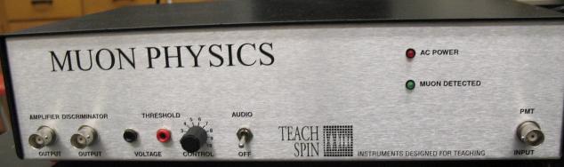
The front panel of the electronics box is shown in figure 5. The amplifier output is accessible via the BNC connector labeled Amplifier output. Similarly, the comparator output is accessible via the connector labeled Discriminator output. The voltage level against which the amplifier output is compared to determine whether the comparator triggers can be adjusted using the “Threshold control” knob. The threshold voltage is monitored by using the red and black connectors that accept standard multimeter probe leads. The toggle switch controls a beeper that sounds when an amplifier signal is above the discriminator threshold. The beeper can be turned off.
 Figure 5- Front of the electronics box.
|
The back panel of the electronics box is shown is figure 6. An extra fuse is stored inside the power switch.
 Figure 6- Rear of electronics box. The communications ports are on the left. Use only
one.
|
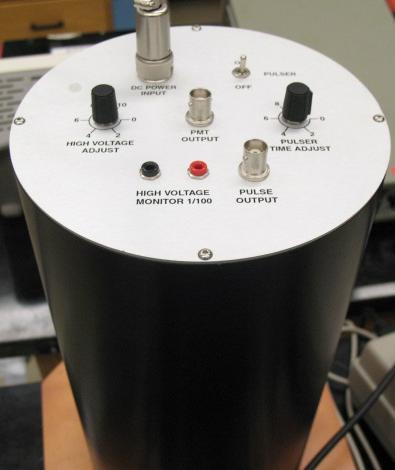
Figure 7 shows the top of the detector cylinder. DC power to the electronics inside the detector tube is supplied from the electronics box through the connector DC Power. The high voltage (HV) to the PMT can be adjusted by turning the potentiometer located at the top of the detector tube. The HV level can be measured by using the pair of red and black connectors that accept standard multimeter probes. The HV monitor output is 1/100 times the HV applied to the PMT.
 Figure 7- Top view of the detector lid. The HV adjustment potentiometer and monitoring
ports for the PMT are located here.
|
A pulser inside the detector tube can drive a light emitting diode (LED) imbedded in the scintillator. It is turned on by the toggle switch at the tube top. The pulser produces pulse pairs at a fixed repetition rate of 100 Hz while the time between the two pulses comprising a pair is adjusted by the knob labeled Time Adj. The pulser output voltage is accessible at the connector labeled Pulse Output.
Software and User Interface
Software is used to both help control the instrument and to record and process the raw data. There is also software to simulate muon decay data. All software is contained in a folder labelled Muon Decay located on the c:\ drive of the computer. There is a shortcut to the main program you will be using located on the desktop called Muon.
 Figure 8- User Interface.
|
There are 5 sections to the main display panel:
- Control
- Muon Decay Time Histogram
- Monitor
- Rate Meter
- Muons through detector
Control
The Configure button allows setting of the communications port. Click on Configure and select com4 located in the Select port section. The maximum x-axis value for the histogram of the muon decay times and the number of data bins is also set here. The default values for these parameters will be used. There are also controls for reading back all ready collected data.
The blue colored Save/Exit switch is used to finalize all your communication and histogramming selections.
 Figure 9- Configure Sub-Menu.
|
The Start button in the user interface initiates a measurement using the settings selected from the configure menu. After selecting it, you will see the “Rate Meter” and the “Muons through detector” graphs show activity.
The Pause button temporarily suspends data acquisition so that the three graphs stop being updated. Upon selection, the button changes its name to Resume. Data taking resumes when the button is selected a second time.
The Fit button will not be used by you. You will fit your data using your favorite fitting package (Mathematica, Matlab, Fortran, Excel, etc...).
The View Raw Data button opens a window that allows you to display the timing data for a user selected number of events, with the most recent events read in first. Here an event is any signal above the discriminator threshold so it includes data from both through going muons as well as signals from muons that stop and decay inside the detector. Each raw data record contains two fields of information. The first is a time, indicating the year, month, day, hour, minute and second, reading left to right, in which the data was recorded. The second field is an integer that encodes two kinds of information. If the integer is less than 40000, it is the time between two successive flashes, in units of nanoseconds. If the integer is greater than or equal to than 40000, then the units position indicates the number of “time outs,” (instances where a second scintillator flash did not occur within the preset timing window opened by the first flash). See the data file format section below for more information. Typically, viewing raw data is a diagnostic operation and is not needed for normal data taking.
The Quit button stops the measurement and asks you whether you want to save the data. Answering No writes the data to a file that is named after the date and time the measurement was originally started, i.e., 03-07-13-17-26.data. Answering Yes appends the data to the file muon.data. The file muon.data is intended as the main data file.
Data file format
Timing information about each signal above threshold is written to disk and is contained either in the file muon.data or a file named with the date of the measurement session. Which file depends on how the data is saved at the end of a measurement session.
The first field is an encoded positive integer that is either the number of nanoseconds between successive signals that triggered the readout electronics, or the number of “timeouts” in the one-second interval identified by the corresponding data in the second column. An integer less than 40000 is the time, measured in nanoseconds, between successive signals and, background aside, identifies a muon decay. Only data of this type is entered automatically into the decay time histogram.
An integer greater than or equal to 40000 corresponds to the situation where the time between successive signals exceeded the timing circuit’s maximum number of 40000 clock cycles. A non-zero number in the units place indicates the number of times this ‘timeout” situation occurred in the particular second identified by the data in the first field. For example, the integer 40005 in the first field indicates that the readout circuit was triggered 5 times in a particular second but that each time the timing circuit reached its maximum number of clock cycles before the next signal arrived.
The second field is the number of seconds, as measured by the PC, from the beginning of 1 January 1970 (i.e., 00:00:00 1970-01-01 UTC), a date conventional in computer programming.
Monitor
This panel shows rate-related information for the current measurement. The elapsed time of the current measurement is shown along with the accumulated number of times from the start of the measurement that the readout electronics was triggered (Number of Muons). The Muon Rate is the number of times the readout electronics was triggered in the previous second. The number of pairs of successive signals, where the time interval between successive signals is less than the maximum number of clock cycles of the timing circuit, is labeled Muon Decays, even though some of these events may be background events and not real muon decays. Finally, the number of muon decays per minute is displayed as Decay Rate.
Rate Meter
This continuously updated graph plots the number of signals above discriminator threshold versus time. It is useful for monitoring the overall trigger rate.
Muons through Detector
This graph shows the time history of the number of signals above threshold. Its time scale is automatically adjusted and is intended to show time scales much longer than the rate meter. This graph is useful for long term monitoring of the trigger rate. Strictly speaking, it includes signals from not only through going muons but any source that might produce a trigger. The horizontal axis is time, indicated down to the second. The scale is sliding so that the far left-hand side always corresponds to the start of the measurement session. The bin width is indicated in the upper left-hand portion of the plot.
Muon Decay Time Histogram
This plot is probably the most interesting one to look at. It is a histogram of the time difference between successive triggers and is the plot used to measure the muon lifetime. The horizontal scale is the time difference between successive triggers in units of microseconds. Its maximum displayed value is set by the Configure menu. (All time differences less than 20 μsec are entered into the histogram but may not actually be displayed due to menu choices.) You can also set the number of horizontal bins using the same menu. The vertical scale is the number of times this time difference occurred and is adjusted automatically as data is accumulated. A button (Change y scale Linear/Log) allows you to plot the data in either a linear-linear or log-linear fashion. The horizontal error bars for the data points span the width of each timing bin and the vertical error bars are the square root of the number of entries for each bin.
The upper right hand portion of the plot shows the number of data points in the histogram. Again, due to menu selections not all points may be displayed. If you have selected the Fit button then information about the fit to the data is displayed. The muon lifetime is returned, assuming muon decay times are exponentially distributed, along with the chi-squared per degree of freedom ratio, a standard measure of the quality of the fit. (For more details[7].)
Exercises
For additional information about the apparatus and more helpful resources about muon physics visit TechSpin.
Apparatus
- "Muon Physics" Scintillator
- "Muon Physics" Control Unit
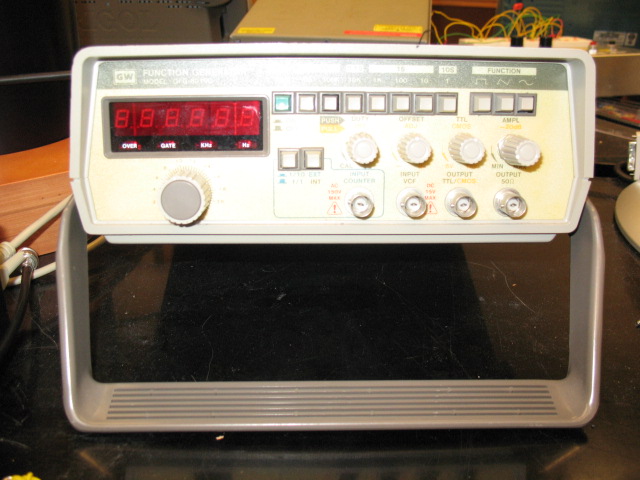
- GW Function Generator (Model: GFG-8016G)
- Digital oscilloscope
- 50-Ω terminators
- Control computer and software
- BNC-to-BNC coaxial cables
Testing the Electronics
You will be using an oscilloscope for the following exercises. Note that every connection into the oscilloscope should be terminated using the provided 50Ω terminator. Log in to the local account on the computer to access the Muon software, using the username and password provided on the top right of the monitor.
Measure the gain of the 2-stage amplifier using a sine wave: Use the oscilloscope to setup a 100 kHz, 100 mV peak-to-peak sine wave on the function generator (FG). (The amplitude knob of the FG should be in the pulled out position to activate the -20 dB internal attenuator. This will allow you to generate the small 100 mV amplitude of the sine wave.)
Connect the output of the FG to the input of the electronics box. Measure the amplifier output and take the ratio Vout/Vin. Due to attenuation resistors inside the electronics box inserted between the amplifier output and the front panel connector, you will need to multiply this ratio by the factor 1050/50 = 21 to determine the real amplifier gain.
Q: Increase the frequency. Over what frequency range does the amplifier operate?
Q: Estimate the maximum decay rate you could observe with the instrument.
Measure the saturation output voltage of the amp.
Increase the magnitude of the input sine wave and monitor the amplifier output.
Q: Does a saturated amp output change the timing of the FPGA? What are the implications for the size of the light signals from the scintillator?
Examine the behavior of the discriminator by feeding a sine wave to the PMT input and then adjusting the discriminator threshold. You can monitor the discriminator output directly on the oscilloscope. Make sure to terminate this connection with a 50Ω terminator as well. Describe the shape of the Discriminator output and explain the behaviour of the discriminator threshhold.
Now we will start looking at actual signals from the PMT. Connect the output of the PMT to the PMT input on the control box. Set the High Voltage Adjust to 10. Run the program Muon on the desktop. Click on Configure and select port com4, then click save & exit. Once you click Start from the Control panel, you will be able to observe the muon count rate in the Monitor Panel.
Adjust (or misadjust) discriminator threshold. Observe the raw muon count rate and the spectrum of "decay" times as a function of the threshold level.
- What high voltage (HV) should you run at? Adjust/misadjust HV and observe amp output. (We know that good signals need to be at about 200 mV or so before discriminator, so set discriminator before hand.) With a fixed discriminator threshold, alter the HV and observe the raw muon count rate and decay spectrum.
- Connect the output of the detector (PMT output) to the PMT input of the electronics box. Look at the amplifier output using the scope.Be sure that the scope input is terminated at 50Ω. What do you see? Now examine the discriminator output simultaneously. Again, be certain to terminate the scope input at 50Ω. What do you see?
Muon Lifetime Measurement
Set up the instrument for a muon lifetime measurement. This is easily done by connecting the PMT output on the detector to the PMT input on the electronics box. You may disconnect the oscilloscope as it is not needed for this part of the experiment. Using the Digital Multimeter (DMM) and the HV 1:100 Monitoring ports on the detector lid set the HV between -1100 V and -1200 V. Next, set the threshold on the electronics box between 180 and 220 mV.
Start and observe the decay time spectrum for several minutes. The average muon rate should be around 6 Hz. The longer this experiment runs for, the more accurate your data will be. We suggest that you collect data over night (or over a weekend) for the best results.
Q: The muons whose decays we observe are born outside the detector and therefore spend some (unknown) portion of their lifetime outside the detector. So, we never measure the actual lifetime of any muon. Yet, we claim we are measuring the lifetime of muons. How can this be?
- Use Ctrl-Alt-PrtScn to obtain a screen capture of the muon main display panel which will include the Muon Decay Time Histogram (you can paste in paint and save file) prior to saving the data. Present this image in your report.
- Using the saved data, recreate your decay time histogram and fit the decay time histogram with your own fitting routine. Describe how you chose bin sizes for the time axis, and how signals due to background events were accounted for.
- From your measurement of the muon lifetime and a value of the muon mass from some trusted source, calculate the value of Fermi coupling constant GF. Compare your value with that from a trusted source.
- Using the approach outlined above, measure the charge ratio ρ of positive to negative muons at ground level.
- Once the muon lifetime is determined, compare the theoretical binomial distribution with an experimental distribution derived from the random lifetime data of individual muon decays. For example, let p be the (success) probability of decay within 1 lifetime, p = 0.63. The probability of failure q = 1 − p. Take a new set of data (different from the one you used to determine the muon lifetime) of 2000 decay events. Group the data, chronologically, in sets of 50 points. (This leaves you with 40 sets of data containing fifty points.) Examine each data set and record how many events, or times, in each of the sets have a lifetime less than the lifetime you found out earlier. (On average this should be 31.5) Do this for all 40 of the data sets. Histogram the number of "successes." The plot of 40 data points should have a mean at 50*0.63 with a variance σ2 = Npq = 50*0.63*0.37 = 11.6. Are the experimental results consistent with theory?
References
- ↑ Most of the information contained herein was taken directly from the manual supplied with the apparatus, Coan, T.E. and Ye, J. "Muon Physics", Muon Physics
- ↑ Simpson, J.A., "Elemental and Isotopic Composition of the Galactic Cosmic Rays", in Rev. Nucl. Part. Sci., 33, pp. 323.
- ↑ 3.0 3.1 3.2 Particle Data Group
- ↑ 4.0 4.1 4.2 Rossi, B., High-Energy Particles, Prentice-Hall, (1952).
- ↑ Wheeler, J.A.,"Some Consequences of the Electromagnetic Interaction between μ--Mesons and Nuclei Rev. Mod. Phys. 21, 133 (1949)
- ↑ Reiter, R.A. et al.,"Precise Measurements of the Mean Lives of μ+ and μ- Mesons in Carbon" Phys. Rev. Lett. 5, 22 (1960)
- ↑ Bevington, P.R. and Robinson, D.K., [https://www.library.yorku.ca/find/Record/1630516 Data Reduction and Error Analysis for the Physical Sciences] McGraw-Hill, (2003).